Patterns of Color Polymorphism in the Intertidal Snail Littorina sitkana in the Race Rocks Marine Protected Area.

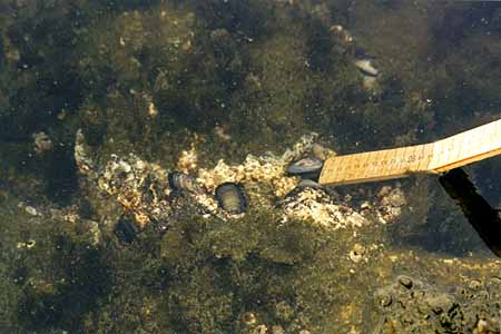
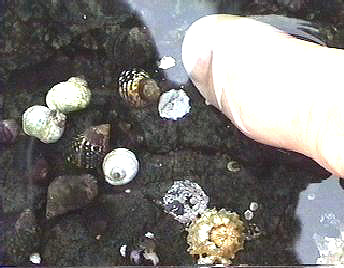
- Figure 1 In Fig. 1 the snails were purposely placed on the white quartz substrate to show the contrast between a shell of color 27 ( white ) and some of colors 1 – 10 ( Black to grey ).
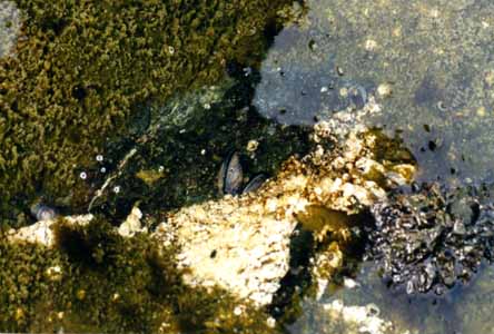
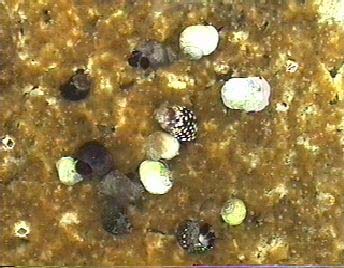
- Figure 2 The same process was repeated in Fig. 2 below only on black, basaltic substrate adjacent in the same tidepool. (Note three black snails (color 1-10) in lower left hand corner.)
- In Figure 3. Several colors of snail can be seen grazing on the golden diatoms in Pool 4 in the spring of 1998.
Extended Essay done by: Giovanni Rosso, Lester Pearson College, 1998 .
The complete version of the research is available in the Library at the college.
Abstract:
As with most intertidal gastropods, Littorina sitkana shows remarkable variations in shell color. This occurs both in microhabitats which are exposed or sheltered from wave action. There seemed to be a close link between the shell coloration of the periwinkle and the color of the background substrate. Field work was carried out on the Race Rocks Marine Protected Area in order to investigate patterns of color polymorphism. Evidence from previous studies was used to support interpretations and understand certain behaviors.
The results showed that in the study site there was a very strong relation between the shades of the shells and the colors of the rocks. Light colored shells stayed on light shaded rocks and vice versa. An interesting pattern was noticed with the white morphs. These were rare along the coast
(only 2%), but were present in relatively high numbers in tidepools of white quartz. From previous experience (Ron J.Etter,1988), these morphs seem to have developed as evolutionary response a higher resistance to physiological stress from drastic temperature changes between tides. Some results showed that the white morph is present in an unexpectedly high percentage at the juvenile stage, but then their number decreases dramatically. As in Etter’s study more research needs to be made on the role visual predators have in this phenomenon.
ROSSO, Giovanni Edoardo 0034 -083
Patterns of Color Polymorphism in the Intertidal Snail Littorina littorea at
the Race Rocks Marine Protected Area.
AN EXTENDED ESSAY PREPARED FOR THE INTERNATIONAL BACCALAUREATE
Candidate number: 0034 – 083 February 1999
Name: Rosso, Giovanni Edoardo
Best language: Italian
School: Lester B. Pearson College of the Pacific
Subject: Environmental Systems
Supervisor: Mr. Garry Fletcher
Table of contents:
Abstract ————————————————————— 3
Introduction ———————————————————- 4
Materials and methods ———————————————- 5
Data analysis ———————————————————- 7
Conclusion ———————————————————– 12
Observations ——————————————————— 13
Evaluation ———————————————————— 16
Suggestions for further studies ———————————— 16
Acknowledgments ——- ——————————————- 18
Literature cited —————————————————— 18
Appendix ————————————————————- 19
2
Abstract:
As most intertidal gastropods, the Littorina littorea shows remarkable variation in shell color. This occurs in both microhabitats that are exposed or sheltered from wave action. There appeared to be a close link between the shell coloration of the periwinkle and the color of the background surface. Fieldwork was carried out at the Race Rocks Marine Protected Area in order to investigate patterns of color polymorphism. Evidence from previous studies was also taken into account to better support interpretations and understand certain behaviors.
The results showed that in the study site there was a very strong relation between the color of the shells and the color of the rocks. Light colored shells lived on light shaded rocks and vice versa. An interesting pattern was noticed on the white morphs. These were rare along the coast (Only 2%), but were present in relatively high numbers in tidepools set in white quartz. From previous experience (Ron J Etter, 1988 ), these morphs seem to have developed, as an evolutionary response, a higher resistance to physiological stress from drastic temperature changes between tides. Some results showed that the white morph is present in an unexpectedly high percentage at the juvenile stage, but then their number decreases dramatically with age. As in Etter’s study, more research needs to be done on the role of visual predators in this phenomenon.
3
Introduction:
There is strong evidence to prove that intertidal gastropods are highly polymorphic for shell coloration (Ron J Etter, 1987). Even within a single species it is not uncommon to find considerable shell color variation in a single trait (Laurie Burham, 1988 ). In the genus Littorina the color of the shell often appears to be parallel to the one of the background (Heller, 1975; Smith, 1976; Reimehen, 1979; Hughes and Mather, 1986 ). Nevertheless the causes and patterns of color polymorphism. in intertidal gastropods are still a fairly unexplored field. Many paths have been undertaken to make some light upon these obscure areas. The most common interpretation was always the presence of visual predators (Ron J Etter, 1987) like birds and fish. Others investigated on the effects of the shells diets. But more recent studies ( Rowland, 1976; Ossborne, 1977; Berry, 1983 ; Etter, unpubl. ) have shown that diet virtually does not affect the shell coloration, although the intensity of pigmentation might be slightly altered. Finally, physiological stress has been introduced as a possible cause color polymorphism. A very interesting study, made by Ron J. Etter on the intertidal snail Nucella Lapillus, shows how the white coloration suffers much less from temperature variations in dry micro habitats as opposed to the brown morphs. With his work he gave some revolutionary insights on the distribution of the shells according to their color.
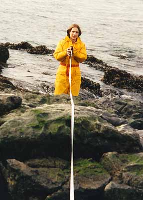
In my fieldwork I chose to disprove the null hypothesis that there is no link between the color of the periwinkle and the color of the substrate it is living on. In order to do this I sampled a great quantity of empty shells and scaled their color from I to 27. 1 then chose five rocky coastal areas, each of a different shade. I analyzed the color of the live shells on each of the chosen rocks, scaled them according to their color and then graphed the results. I also observed the young shells in the inside of barnacles and took notice of their color frequencies in relation to their quantity. I ended my study looking in some tide pools and recording new surprising results. I concluded that:
There is a link between the color of the shell and the background color.4
I roughly calculated that between one station and the other there was a change in tide level of 13 cm. I therefore kept this in account and lowered the quadrat accordingly into the water.
Data analysis-
Rock – 1 (Black)
The rock contained a creek were I noticed a very high density of periwinkles in a very limited area. In the inside of the creek they were almost piled and glued on top of each other. With the help of a pen I extracted them and laid them on a white sheet of paper. Once I accomplished the process of identification I put them back. I noticed that the bigger shells (10 to 14 mm wide) were located on top of the smaller ones (3 to 6 mm wide). This made me think that the bigger ones wanted to protect the smaller ones from swells and predators. It actually does work as a protection system, but it surely is not because of the kind nature of periwinkles. It is obviously a matter of physical size.
Rock #1 -Shade #1
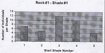
From the graph we see that the black rock hosted the darkest shades, from 1 to 5. The average number of individuals per shade is 7.6. The average shell color is 3.
7
Rock # 2- Dark grey
As opposed to the previous case the surface of rock # 2 was rather flat. Population was regularly distributed. All shells seemed to be above 5 mm in width. Here I had the opportunity to understand the great resistance that periwinkles have to salinity changes. In fact some of the shells were located under the flow of a fresh water pipe. It might have been a coincidence but these shells were slightly bigger (7 to 12mm wide).
Rock #2 – Shade 2
. 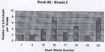
The graph shows that there are some exceptions (Color 1, 3) to the trend that has been shown in the previous graph. I guessed that these are the cases of lucky shells that have not jet been seen by birds or fish. The average number of individuals per shade is 4.25 . The average shell color is 13.6 .
Rock – 3 (Brownish red)
The reddish color of the rock came from many small algae that covered its surface. I did not notice any irregular patterns in distribution. The shells seemed to be above 5 mm in width.
8
The background color was parallel to the shade of the periwinkles. Color 1 and 20 appear to be exceptions: only three individuals in total. The average number of individuals per shade is 4.4 . The average shell color is 9.4.
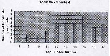
Rock – 4 (Light brown)
Rock #3 -Shade 3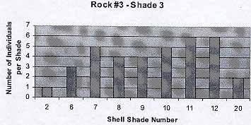
The surface of the rock was very irregular.. Some areas were covered with dead barnacles ( Balanus sp. ). I noticed that here the shells were smaller in size and they tended to be gathered around the barnacles. Nevertheless I repeated the process.
Rock #4 -Shade 4
9
The population reflects the previous trends. The average number of individuals per shade is 3.8. The average shell color is 11.3.
Rock – 5 (White rock with dark patches)
This rock was one of the most interesting ones. In fact, the two different shades of the rock gave place to a particular phenomenon that clearly disproved the null hypothesis. I tried to be as precise as I could in distinguishing the shells on the white and dark spots. I noticed the net distinction between the color polymorphism on the two areas.
Rock #5 -Shade 5
In the light patches the average number of individuals was 4.3. The average shell color was 23. In the dark areas the average number of individuals was 4.8. The average shell color was 3.
If the color of the shell would be directly proportional to the one of the rock, the average shell colors would be:
Ideal Model
10
Rock 1
|
| 3 |
| Rock 2 |
13 |
| Rock 3 |
8 |
| Rock 4 |
18.5 |
| Rock 5 |
24.5 / 3 |
Actual Model
In the actual experiment the averages were:
Rock 1
|
| 7.6 |
| Rock 2 |
13.6 |
| Rock 3 |
9.4 |
| Rock 4 |
11.3 |
| Rock 5 |
23 / 4.8 |
I assume that the dark grey rock is actually lighter than the brownish red
one. If we observe the results we understand that that:
|
Rock Number
Actual Shade |
Ideal One |
Error |
| 1 |
7.6 |
3 |
4.6 |
| 2 |
13.6 |
13 |
0.6 |
| 3 |
9.4 |
8 |
1.4 |
| 4 |
11.3 |
18.5 |
7.2 |
| 5 |
23 / 4.8 |
24.5 / 3 |
1 / 1.8 |
Considering that a minority of the shell color numbers was far away from the average: the average error is of 2.8. This means that on average the actual color was 2.8 units away from the ideal one, therefore disproving the null hypothesis. (Chi square test was used to verify the results.)
11
Conclusions:
The data analysis clearly shows that in the Race Rocks area there is a very strong relation between the color of the shell and the color of the background they are standing on. The shells with light shades are found on light colored rocks. The same relation is true also for the opposite extreme case were we find black shells on black rocks.
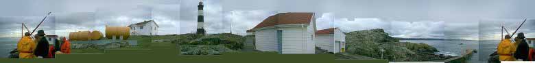
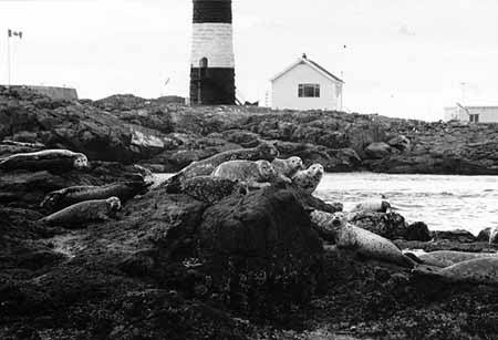
I feel that the model we can create from this experience is relevant above all because the consequences of human presence are reduced to very low levels. In fact, I have been operating in a Marine Protected Area were not many people go. The area is relatively free both from water and air pollution. The only predators are the natural ones. Besides this, the ecosystem is intact and the populations of all the organisms are at almost climax level. The amount of visual predators includes crabs, sea gulls, black oystercatchers, pigeon guillmonts, otters and fish.
From the observations made (p. 13, second part) on the entirely white morphs, we may deduce that there is a strong link between what Ron J. Etter found out on the Nucella lapillus and the Littorina littorea. Putting the pieces of the puzzle together we notice that the distribution of periwinkles is obviously affected by numerous reasons. There seems to be a wide color gap between the shades 1 to 26 and 27. The first twenty-six, when wet, are not very different from each other. The white morph instead is clearly identifiable both when it is wet or dry. If we keep in account that the vast majority of the coastal area on Race Rocks is dark, obviously it will be easier to for shells 1 to 26 hide. The white shells instead have such a great disadvantage that only 2% survive. Keeping in account Etter’s results we may conclude that, excluding a minority of extraordinary circumstances, all these deaths are caused by predators. In fact, when the juvenile periwinkles leave the barnacles, their shell is still soft. Now, if the white periwinkles are born near an area of white surface, then their chances of being seen decrease and actual groupings of white shells may be noticed. The color of their shell also allows them to bare physiological stress much better than the darker shades. The stress comes from the drastic changes in temperature between tide variations. In the case of the Nucella lapillus, in Etter’s experiment, the white shells inhabited most of the sheltered areas and, as previously mentioned, dry areas. This could also apply to the Littorina littorea, but on the Race Rocks Island the sheltered areas are very few and the number of predators is high. The white quartz is the only substrate that can host them (once they leave the Balanus sp.). I feel that if the ocean conditions were not as rough and there would be fewer
12
predators, the white morphs would also be seen on the darker rocks. In the tide pool both the white morph and the dark one live together The mortality of the last though is obviously higher, both for predation and stress (Ron J Etter).
In the dark areas the presence of the white morph is almost nonexistent (2%). But the shells belonging to shades 1 to 26 are distributed according to a remarkable pattern. On light colored rocks we will find shells that belong to the high numbers. In the opposite case the same trend applies. – In the area I took in exam this close relation is probably emphasized by the high intensity of predation. The contrasts are easily spotted and eliminated. Therefore, in the absence of predators, I think that the darker shells would be able to live on any color surface. Of course the dark population would suffer more in the dry areas as opposed to the lower levels.
Observations:
As I was watching the newborn shells (about 1 mm wide) in the dead barnacles I found out that the presence of white shells is unexpectedly high at this stage. I tried counting them and recording the results. On average a dead 20-mm wide Balanus sp. holds between four and eight shells of Littorina littorea. I analyzed ten samples in two different areas and recorded the number of white juvenile shells:
Area
|
| Total number of shells |
Number of white shells |
| 1 |
5 |
2 |
|
6 |
2 |
|
8 |
4 |
|
4 |
3 |
|
4 |
1 |
|
5 |
3 |
|
6 |
4 |
|
7 |
3 |
|
6 |
2 |
|
8 |
5 |
| 2 |
4 |
2 |
|
7 |
4 |
|
8 |
5 |
|
3 |
0 |
|
5 |
3 |
|
7 |
4 |
|
8 |
4 |
|
6 |
3 |
|
4 |
3 |
|
9 |
5 |
In the first area the average Balanus sp. held 5.9 periwinkles and 2.9
were white or very light colored. The percentage of white shell was of 49.
In the second area the average Balanus sp. held 6.1 periwinkles and
3.3 were white. The percentage of white shells was of 54.
The results show that on average 51.5% of the shells are white. If we
make an exception for the tidepools, the percentage of white shells present
on the protected coastal areas is 2 (This is an approximate calculation made
when collecting the dead samples and when counting the live ones). This
means that 49.5% are eaten or die before reaching a sufficient size to move
in an area where they would be protected by the background they are
standing on. According to the study made by Ron J. Etter on the intertidal
snail, Nucella lapillus, when the brown morphs and the white ones were put
on the same exposed coastal area, there were virtually no differences in the
mortality rates of the two. If we dare to make a parallel between the two
species, it would be therefore wrong to assume that the white morphs die
because of natural causes such as diseases or disadaptation. It is my opinion
that literally 49.5% of the white morphs is victims of visual predators
because they can easily be seen before reaching an area where they would
camouflage. In this case, I am not including tide pools with white bottom
and where the water is shallow. I am referring to the morph with shade 27,
which is not common along the coast probably because of the lack of
almost entirely white rocks.
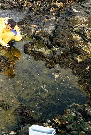
On the other hand I mentioned tied pools because of a specific reason. In
fact, on the Southwestern part of the island there are six tide pools, each
with different depths and different consequent bottom coloration. During
the days of the experiment this area was inaccessible for the presence of
about 75 California sea lions and about 23 Stellar. Nevertheless, in previous
visits to the island for other reasons (the reserve is in fact managed by
Pearson College and is used for several academic programs, projects and
environmentally oriented diving) I had the opportunity to observe the
presence in tide pool – 4 of about 20 entirely white shells of Littorina littorea
standing on white quartz. This had originated a question that had long
14
remained without an answer. Why can the white periwinkles be found only in this tide pool (if we exclude the two- percent I was talking about before)? The most common explanation was based on the presence of certain minerals, difficult predation and a genetic mutation that occurred only there. To be honest, after coming across Ron J. Etters study on the Nucella Lapillus, it was hard for me not to relate the two cases.. In his study he states that the white morph heats up at a lower rate as opposed to the brown morph in shallow and protected areas. Observing a higher rate of mortality (not due to predation) in the brown morph, he deduced that the white morph had developed a better defense mechanism against physiological stress. It therefore has higher chances of survival in very shallow water or in those areas that remain exposed between tides for a long time. Although brown snails can avoid exposure to the sun by moving to more shaded and moist microenvironments, Etter thinks their greater susceptibility to stress nonetheless puts them at a disadvantage by limiting their foraging area and increasing the amount of time that they must spend in hiding- This in turn could lead to slower growth rates and reduced levels of fecundity (Laurie Burnham, Scientific American, September 1988 ). On the other hand this does not exclude the presence of natural predators, especially in young age.
If we compare these results to the observations made on Race Rocks we may find many points in common. Especially after I had a new confirmation. In fact, in a tide pool with difficult access in another part of the island I found a similar behavior. On a small area of white quartz I found five entirely white periwinkles. There is a big difference in size between the ones I found there and the population of tide pool – 4. The first ones were about 2-3 mm wide; the second ones were 6-12mm. This might be due to the fact that they were living in a creek of difficult access to most predators. Nevertheless the pattern fits: the white periwinkles are almost all found in areas of shallow water or that remain exposed for a long time between the action of tides. On the other hand these are the only areas were white quartz is found on the island. The observations made on the fieldwork make me almost certain that the reasons for the white morphs to be in the tide pools are an adaptation to physiological stress and a perfect camouflage. In Etters experiment most of the protected areas were inhabited by white morphs. On Race Rocks only two tide pools contained such organisms and in very low quantities. I think this can be explained by the combination of several factors. In the first place the ocean conditions around the island are
15
very rough and they make it hard for the shells to survive in all areas.. In the second place there is very limited quantities of white rock were the shells can camouflage. Finally the very high quantity of visual predators, both from the air and form the sea, make it very difficult for these shells to move around because they will immediately be seen.
Evaluation:
Due to the lack of hi-tech material I had to verify my observations with simple tools- This forced me to use other people’s previous studies (Ron J. Etter) to better understand what I saw. If I had disposed of an instrument to measure the internal temperature of the shells I could have repeated Etters experiment on the Littorina littorea.
My experiments allow the creation of a model that is true, as far as we know, only on the Race Rocks Marine Protected Area. Other generalizations should be verified. In order to obtain a more reliable model the experiment should be repeated over a longer period of time on a regular basis. The month of October is a period when there is a significant increase in predation also due to the fact that the colony of seagulls on the island is incremented by the newborn.
I chose a vast scale of shade variations in order to achieve more precise results. By doing this, it was hard for me to identify exactly to which number each shell belonged. Even though I tried my best I might have made some mistakes.
Knowing that there are significant differences in distribution between the exposed and the sheltered areas, each of the sites was not exposed to the same environmental conditions. Some were more exposed to currents than others.
Suggestions for further studies:
As I mentioned in the introduction the causes and patterns of color polymorphism in intertidal gastropods are a fairly unexplored field. There are therefore still many grey areas that need to be cleared.
The fieldwork I had the opportunity to make on Race Rocks allowed me to learned many things on these fascinating creatures, but posed also many questions to which I have no answer.
I was surprised when I found so many white periwinkles in the barnacles. It would be interesting to find out exactly what happens to them once they leave these shells:
Who exactly are their predators?
16
At which stage in growth does their shell become too hard to be digested?
How do they choose the areas where they stop?
Are there certain types of minerals that create better conditions for living? Is there a link at all?
What is the exact probability for a shell to be white at birth?
Is the gene universal or is it majority- present in certain areas?
How does the alimentation affect growth and reproduction rate?
The white shells are more tolerant to physiological stress, but does this affect the immunitary system? Which diseases are the most common?
The fieldwork I have done seems to apply for Race Rocks, but is it true also in other nearby areas? To what extent does the exposure to rough environmental conditions affect distribution? Since the tide pool was covered and surrounded by sea lions, it was obviously affected by their waste products. The population of periwinkles seems to be fairly stable? How tolerant are these shells to changes in pH? Is there a difference between the degree of tolerance of the dark and the white morphs?
17
Acknowledgments
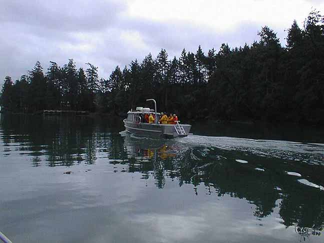
I sincerely thank my supervisor, Mr. Garry Fletcher, for his encouragement, support, precious advise and constructive criticism. I am also very grateful to Mr. Mike and Miss. Carol Slater for hosting me on the island during the field work. I will never forget the delicious supper we had together on Thanksgiving Day. In the end, I would like to thank Mr. Chris Blondeau for his sincere interest and for bringing me at Race Rocks by boat.
Literature cited:
Laurie Burnaham, September 1988, The hard shell, pp.26-27, Scientific American.
Ron J. Etter, April 1987, Physiological stress and color polymorphism in the
intertidal snail Nucella Lapillus, Museum of comparative zoology, Harvard
University, Cambrige, MA 02138.
Jane M. Hughes and Peter B. Mather, December 1984, Evidence for predation as a
factor in determining shell colorfrequencies in a Mangrove snail Littorina Sp.,
School ofAustralian Environmental Studies, Griffith University, Nathan,
Queensland,Australia.
18
APPENDIX 1. Photographs of Littorina littorea
In Fig. 1 the snails were purposely placed on the white quartz substrate to show the contrast
between a shell of color 27 (white) and some of colors
1 – 10 ( Black to grey).
The same process was repeated in Fig. 2 below only on black, basaltic substrate adjacent in the
same tidepool. (Note three black snails (color 1-10) in lower left hand corner.)
Figure 1 Figure 2
19
Apendix 2. Photographs of the shell shades of Littorina littorea
There was a very significant difference in color between the dry and the wet shells. In the two pictures some of the shells had to be moved around in order to maintain the darker periwinkles before the lighter ones. For example, wet shell number 11 had to be moved to 9 on the dry scale
20
Appendix 3. Picture from Ron J. Etters fieldwork
Ron J. Etter noticed that in the Nucella Lapillus the white morph was more common in the sheltered areas. The brown one dominated in the areas of wave exposure. He concluded that the color of sea shells on the seashore may be an evolutionary response to physiological stress.
The color of seashells on the seashore may be an evolutionary response to physiological stress
Photographs of Littorina sitkana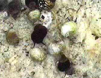 Figure 1
In Fig. 1 the snails were purposely placed on the white quartz substrate to show the contrast between a shell of color 27 ( white ) and some of colors 1 – 10 ( Black to grey ).
The same process was repeated in Fig. 2 below only on black, basaltic substrate adjacent in the same tidepool. (Note three black snails (color 1-10) in lower left hand corner.)
 Figure 2
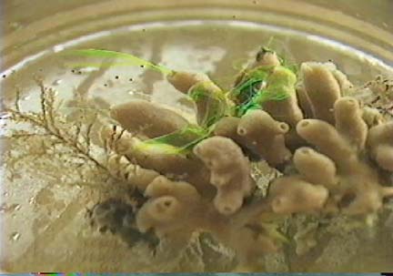
 In Figure 3. Several colors of snail can be seen grazing on the golden diatoms in Pool 4 in the spring of 1998.