Snow as an Abiotic factor at Race Rocks

Every few decades, Victoria receives very large snowfalls, including the more than 100 cm (39 in) of snow that fell in December 1996. On the other hand, roughly one third of winters will see virtually no snow, with less than 5 cm (2 in) falling during the entire season. When snow does fall, it rarely lasts long on the ground. For Victoria Harbour, the climate records report annual mean snowfall totalling 29.3 cm ( about a foot) falling on 8 days..The Environment Canada website lists Victoria ( Airport ) as the city having the fewest snow days of all cities in Canada (10) The mildest winter (7.4 degrees average) and the lowest snowfall (43.8 cm.)The headlines in the Victoria Times for November 27, 2006 read :

“Snow shutdown
Schools closed, buses delayed
Victoria Times-Colonist
Published: Monday, November 27, 2006
Snow has shut down much of Greater Victoria.
Public schools in Saanich, Victoria and Sooke are closed, as are many private schools and the region’s major post-secondary institutions, including University of Victoria, Royal Roads University and Camosun College. “

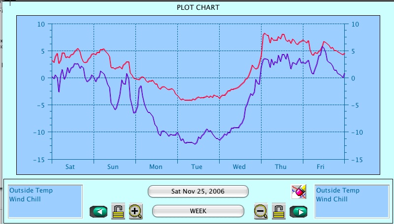
The snowstorm of November 26, 2006 can be traced from the Victoria harbour data on the Environment Canada website. Here it can be seen that the snow started on the morning of November 26 and continued until early morning of the next day. It snowed again midday on the 29th of November . The temperature that week took an unseasonal plunge.

On Race Rocks our weather station recorded the windchill from the North East pushing the temperature down to minus 13 degrees Celsius
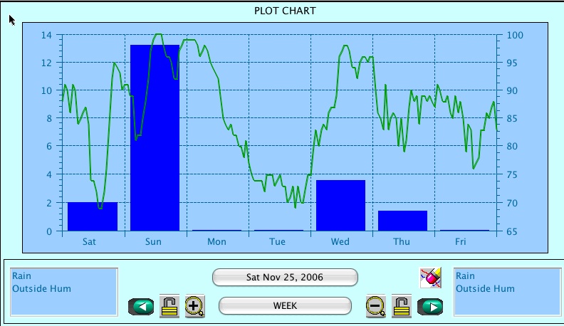
The blue bar represents rainfall, with the scale in mm.on the left. The green line is humidity. After Sunday, the freezing temperature prevented the instrument from registering rain. for several days. Due to blowing snow, it is unlikely that all snow that fell was measured..
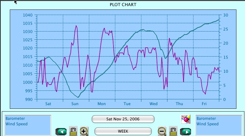
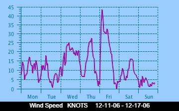
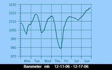
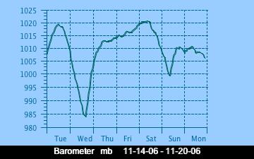
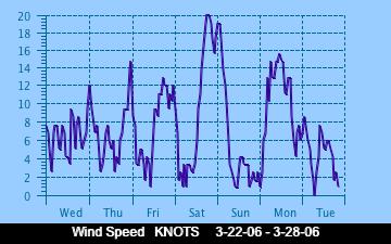
Wind speed is the purple line, and barometer is the blue line. Note how the barometer plunged just as the snowstorm started. The wind remained high for most of the week. This graph represents the surface wind profile. At the top of the tower it averaged 10-15 knots higher.

THE ABIOTIC EFFECTS OF SNOW:
Our second snowfall for the year arrived on January 10, 2007. Pam Birley took this photo for us. This was unusual for Victoria as we had been smugly assuming that we had already had our share of snow that stayed for a week for the winter.

No research has been done at Race Rocks on the effects of snow on the animal and plant life other than the observation that the birds disappeared while these severe storm events were in progress. It is also almost impossible to access Race Rocks during a snowstorm since the wind blows in from the north-east and the exposure at the jetty prevents a boat from landing.


See the exercise on the water cycle

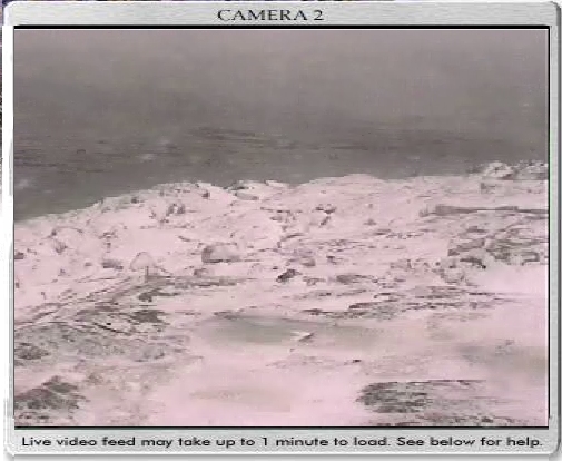
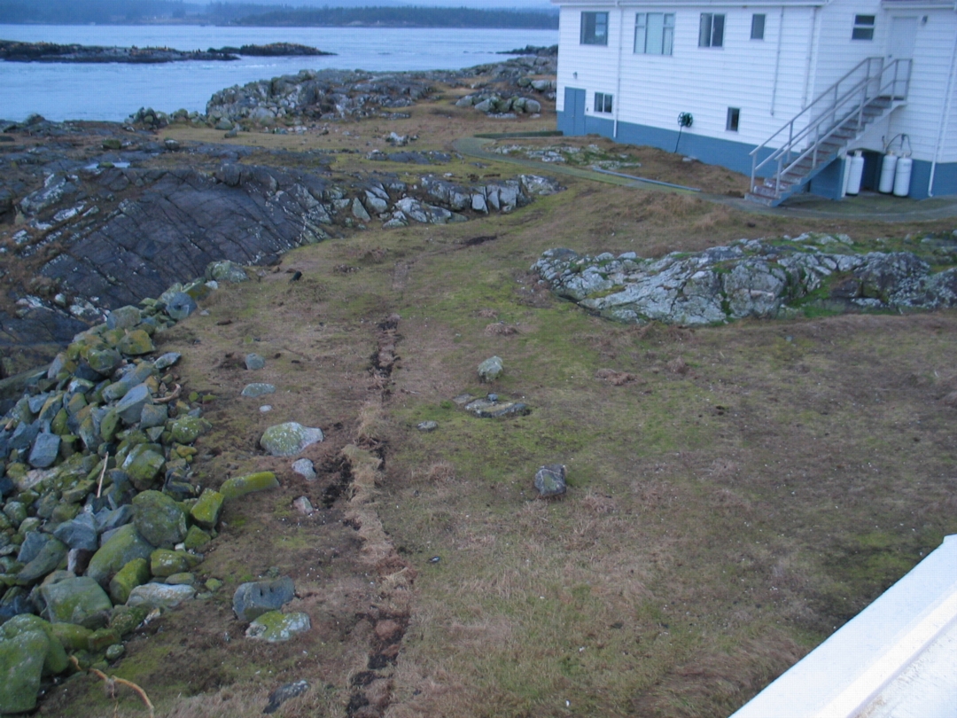
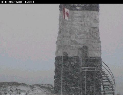
This image from the webcam in the November, 2006 snow storm showed a bleak landscape, with no seagulls in the usual spot. In a week they had all returned however, as mild temperatures returned.

The topic of SNOW ECOLOGY has not been extensively studied. One of the classic works on the topic was done by William Pruitt of the Department of Biology at the University of Manitoba.
This paper is available from the TAIGA BIOLOGICAL STATION THESES AND RESEARCH PAPERS
( Formozov-inspired Concepts in Snow Ecology in North America. Bulletin Moscow Society of Naturalists, vol.104, No.3:pp.13-22. William 0. Pruitt, Jr.)

Records of snowfall from 1985 to February 1996 may be found on the Environment Canada Website Search that website for total snowfalls during that period click on British Columbia/advanced search/ then enter Race Rocks in the Search by Station Name section. Use the pull down menues to find the year, month or day of interest
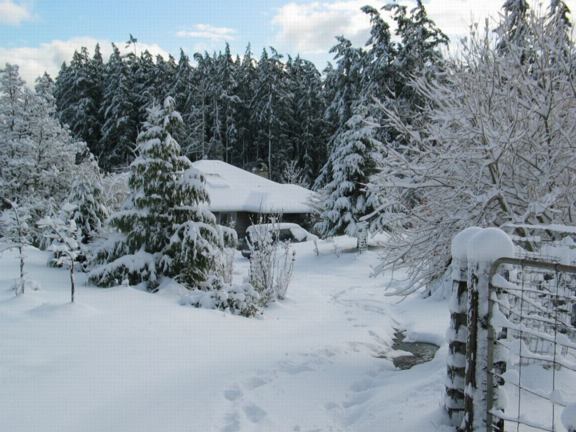
In nearby Metchosin, by November 27, 2006, over 40 cm of snow blanketed the forests and farms. A week later, the snow had all but disappeared. Considerable damage to tree branches was sustained during this snowfall.
Extreme Weather Events at Race Rocks

How We Got Blasted: Record-ripping winds took rare path:

Judith Lavoie, Times Colonist Published: Saturday, December 16, 2006

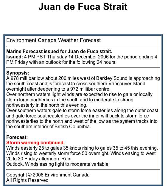
Wind gusts at Race Rocks, off the Island’s southwest tip, reached a record 158 kilometres an hour as the third intense wind storm in a week plowed a trail of destruction through southern Vancouver Island and the Lower Mainland. Yesterday morning’s storm knocked out power to thousands of residents, toppled trees, and damaged buildings and cars. More residents were forced from their homes because they didn’t have power, and ended up moving into hotels or into the homes of friends and relatives. Around the capital region, areas that suffered the most damage had winds that gusted to between 70 and 90 km/h . In the last three storms, including yesterday’s, the wind has gathered over the North Pacific, whooshed across the ocean, gathered speed in the funnel of Juan de Fuca Strait and then whacked Vancouver Island with its full force, said Chris Emond, Environment Canada meteorologist. “There are tremendous wind speeds and three in one week is unusual.” The wind is coming straight across the cold North Pacific and hitting land, rather than taking the more common route of dipping south and picking up tropical moisture, Emond said.

Anne McCarthy, weather services specialist with Environment Canada, said the storms are cutting a swath straight across Vancouver Island instead of the more usual pattern of tracking to the north coast around Prince Rupert and the Queen Charlottes (Haida Gwaii.) Although we have only recorded extreme values since earlier this year, It is interesting to note the Maximum wind and the Minimum Pressure records for the 14th and 15th of December 2006.

You can read the complete story in the Times Colonist , Dec 16, 2006 The right conditions for a hurricane:

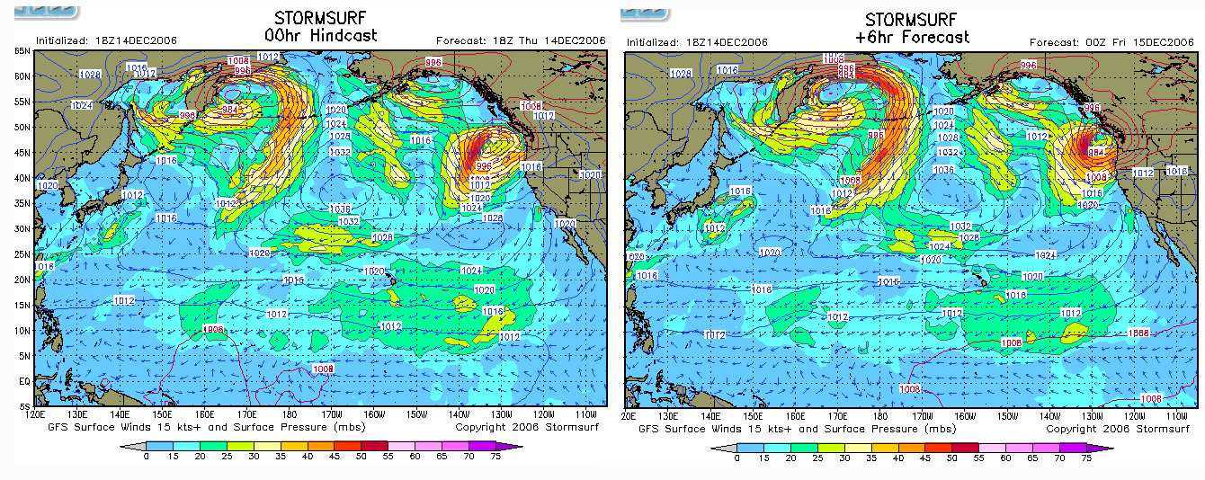
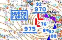
Storm surf conditions which correspond to the low pressure systems. These images were captured from the Stormsurf site at 2300 hrs. Pacific Time , just a few hours before the maximum impact.

This image was taken from the US National Weather Service Images of the evening of December 14. Note the “HURRICN FORCE” location right beside Vancouver Island. Also the atmospheric pressure is as low as 970.

Current Satellite imagery is shown on this page

Return to the Physical Factors Index

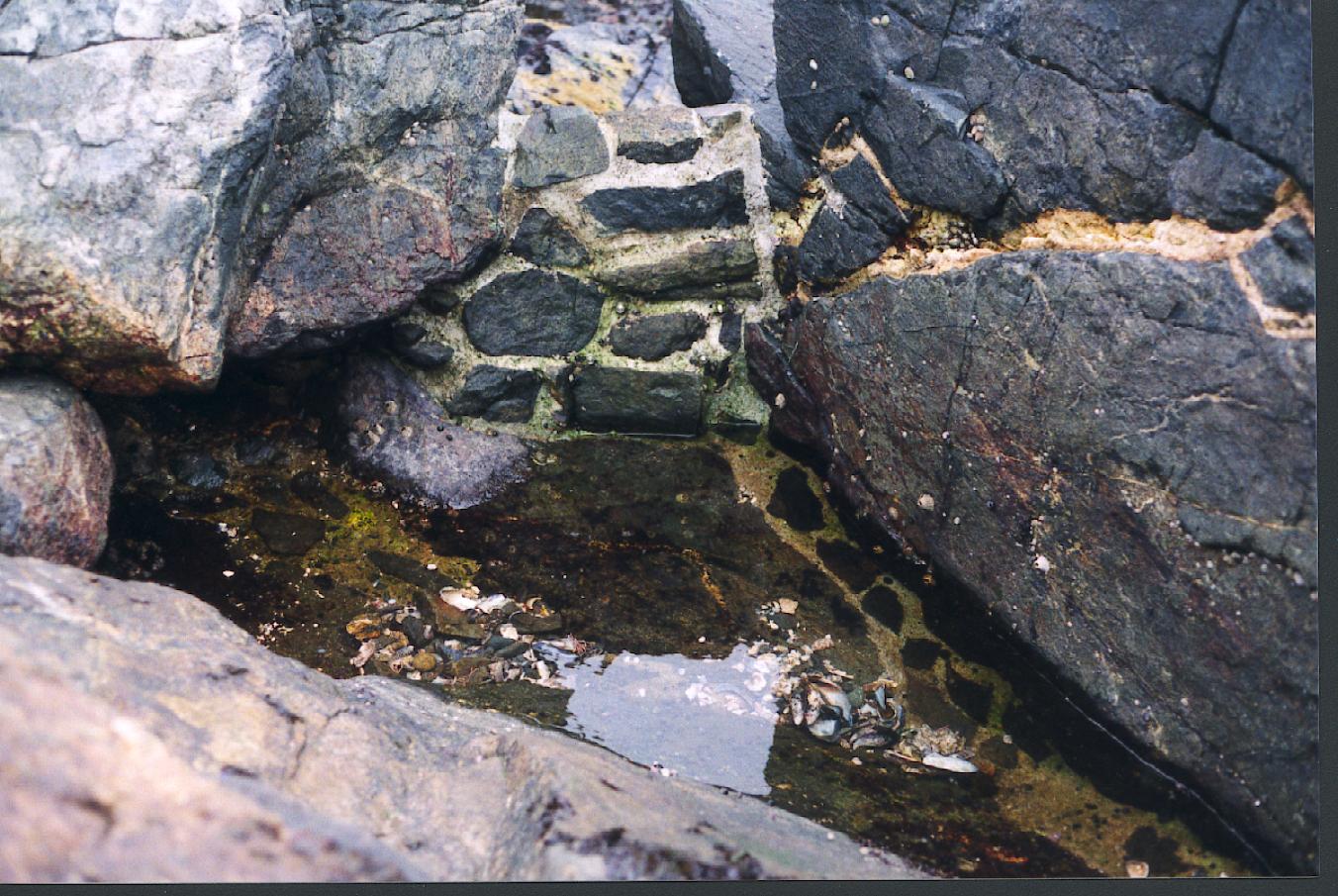
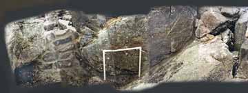
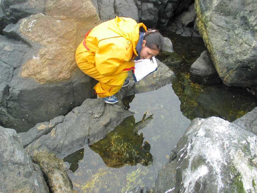
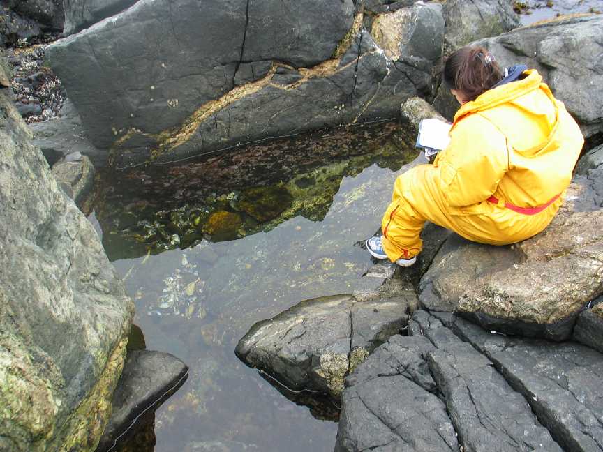
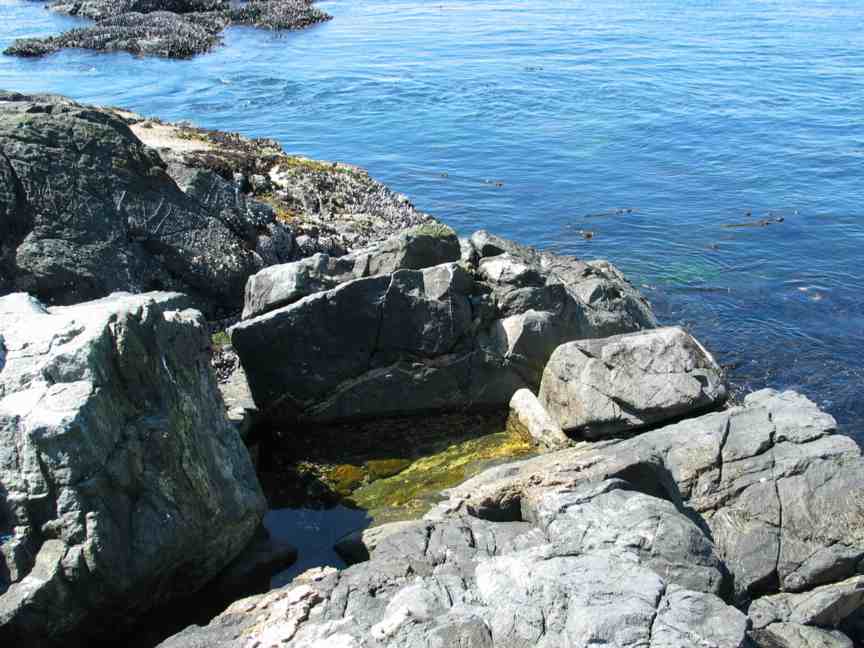
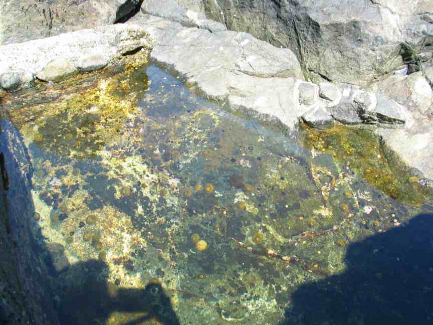
Artificial Tidepool #13 peg #5

The rockwork done to seal the southern entrance

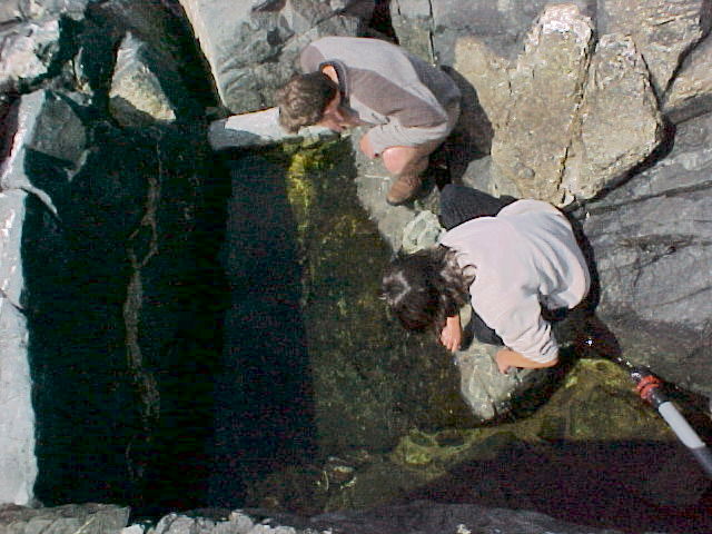
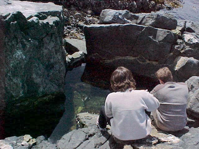
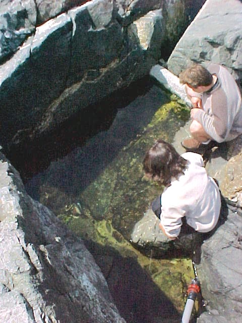
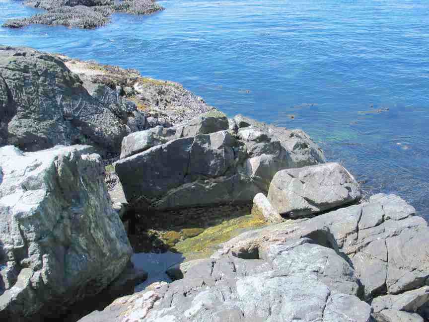
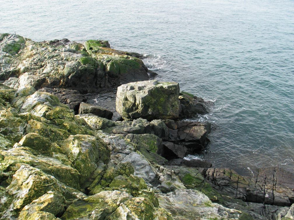
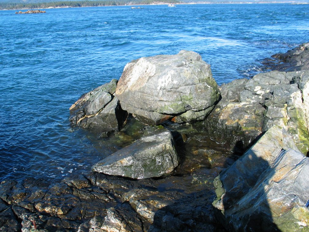
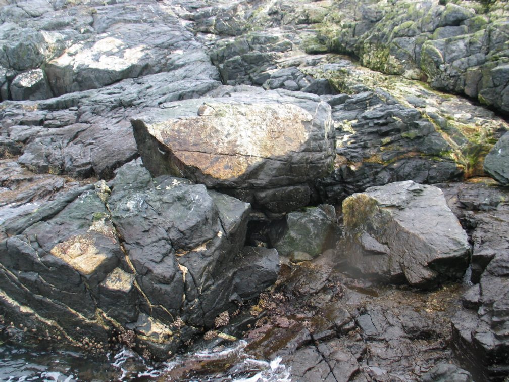
This artificial pool was made under permit from BC Parks by Mike Slater and Garry Fletcher in June, 1999. It is part of a long range succession study.
See also below for “AFTER the HURRICANE”

AFTER THE HURRICANE OF DECEMBER 15, 2006  (newspaper item)

Correlation : Wind and Barometric Pressure Relationships

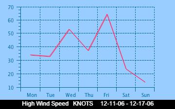
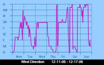
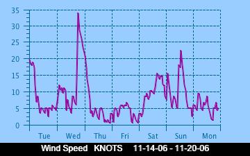
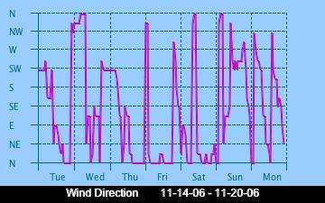
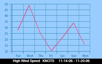
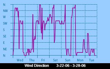
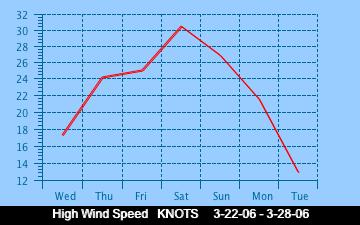
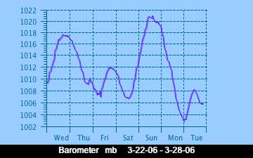
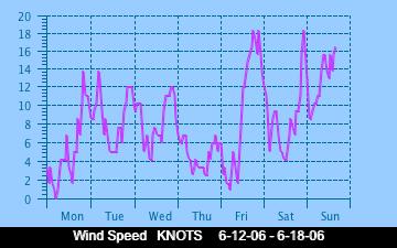
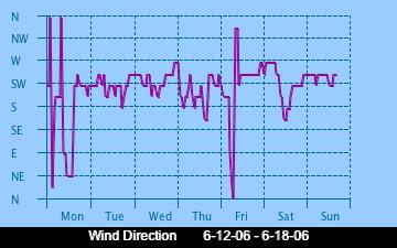
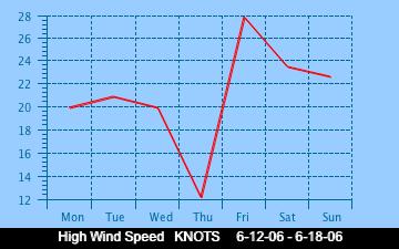
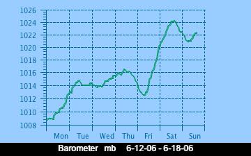
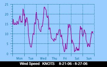
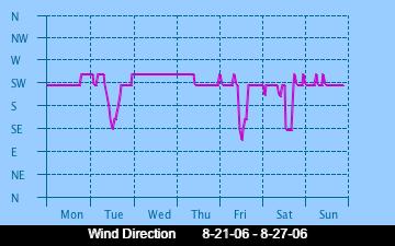
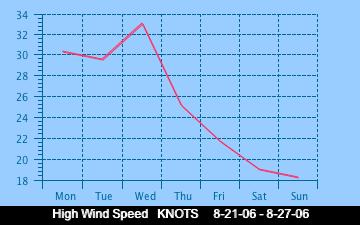
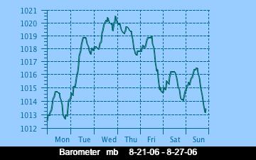
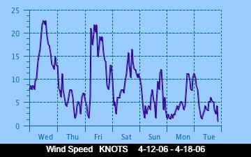
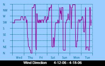
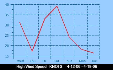
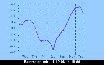
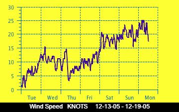
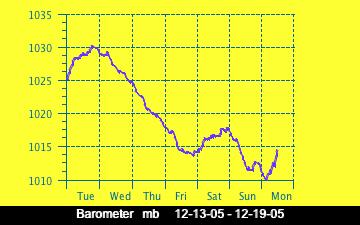
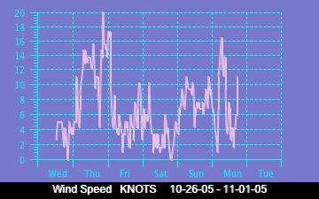
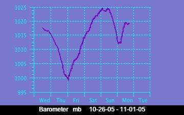
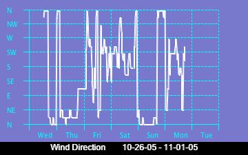
Below are presented some of the historical graphs of wind direction, wind speed and barometric pressure as recorded on the weather station at Race Rocks. . Several interesting problems can be posed from which one could form some hypotheses using these data. Make a similar comparison with the current week’s graphs.

Note: you may find some variations in patterns in the summer.

Lightning as an Abiotic Factor at Race Rocks

Lightning is a very rare occurrence on this part of the Pacific North West Coast, however we show below a method of recording lightning strikes which can be used to compare with other regions of North America. The unusual thing about lightning is that it can occur here in the Strait of Juan de Fuca in what is the winter months in North America. When lightning is never recorded in the interior…at least of Canada.
We are interested in noting Lightning as an abiotic factor because it contributes to the sum total of Atmospheric Nitrogen Fixation and is therefore an important feature for all organisms which are dependent on nutrients from the Nitrogen Cycle. Nitrogen fixation involves Nitrogen, which is a relatively inert gas, which is plentiful in air, being made to combine chemically with other elements to form more reactive nitrogen compounds such as ammonia, nitrates, or nitrites.
This space is reserved for the first person to record a lightning strike from the remote control cameras at Race Rocks!
OBJECTIVES: After doing this assignment, students will be able to:a) Find out where lightning strikes are presently occurring in North America.
b) Evaluate the importance of lightning in the Nitrogen Cycle.
c) Enumerate the other abiotic effects on organisms of lightning strikes.

Procedure:1. The enormous energy of lightning breaks nitrogen molecules and enables their atoms to combine with oxygen in the air forming nitrogen oxides. These dissolve in rain, forming nitrates, that are carried to the earth. Atmospheric nitrogen fixation probably contributes some 5– 8% of the total nitrogen fixed. See the table below for a comparison of sources of Nitrogen Fixation. The major conversion of N2 into ammonia, and thence into proteins, is achieved by microorganisms in the process called nitrogen fixation (or dinitrogen fixation). Give examples of how this process is essential for life. Include the connection between the muscle in your arm and the process of Nitrogen Fixation.

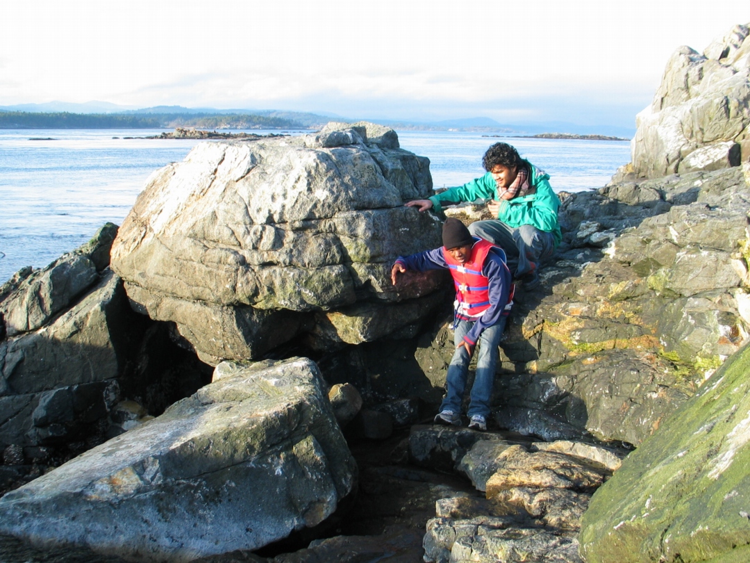
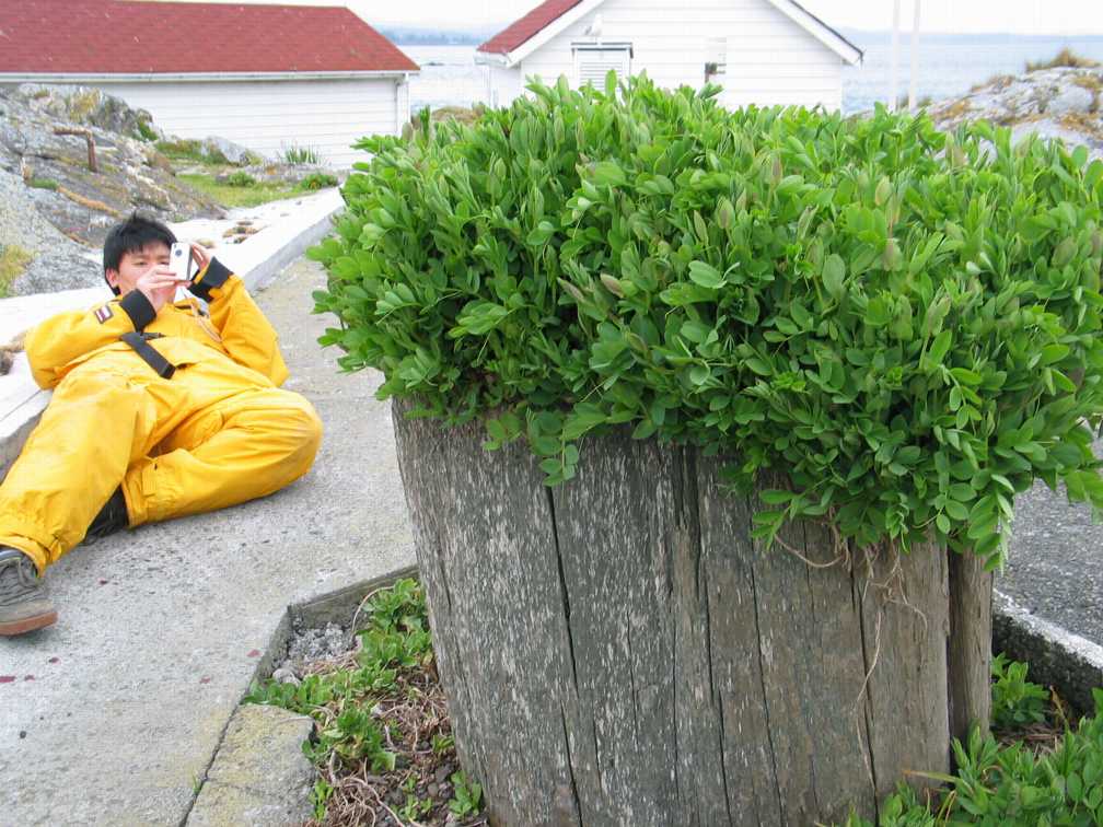
In this picture.. Alex Chan PC yr 32 is trying to get the nitrogen fixing Lathyrus or Beach Pea lined up with Tower at Race Rocks. Check the Beach Pea file to see how well he did.

2.See the file on Biogeochemical Cycles , and construct a Nitrogen cycle from the Race Rocks image clips.

3. The Weather Office of the Government of Canada presents updates of the lightning strikes in North America

Record the Frequency and Location of Lightning strikes on three separate days when you view this link.

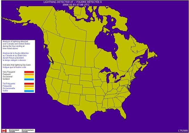
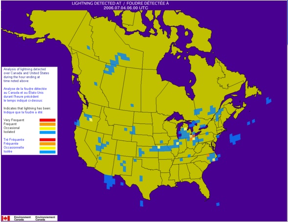
4. Click on the prerecorded sample maps below which show the location and intensity of lightning strikes in the area of the Strait of Juan de Fuca over the period of an hour. In the legend to the left, the estimated frequency of Lightning is depicted as flashes per 1000 square km* per minute as follows:

  • Very Frequent (Red) = more than 6 per minute
  • Frequent (Orange) = 3.0-5.9 per minute
  • Occasional (Yellow) = 1.5-2.9 per minute
  • Isolated (Blue) = less than 1.4 per minute

Note*: 1000 square km represents a circle having a radius of 17.8 km

In the image to the right, you can see the contrast in frequency and intensity of strikes on a July evening. “>
January 31, 2006 2300 hrs
July 3, 2006 1100hrs
The Data below is from various sources, and has been compiled by DF Bezdicek & AC Kennedy, in Microorganisms in Action (eds. JM Lynch & JE Hobbie). Blackwell Scientific Publications 1998. It appears in the website: The Microbial World: N2 fixed (1012 g per year, or 106 metric tons per year)
Type of Fixation
Non-Biological
Industrial about 50
Combustion
about 20
Lightning————–Compare with these other sources ——————-> about 10
Total about 80
Biological
Agricultural land
about 90
Forest and non-agricultural land
about 50
Sea
about 35
Total about 175
5. Extension..for further investigation: Find out why lightning is rare in the winter time in North America, but common in many areas in the summer. If you are from one of these areas that experience many lightning strikes, determine why they are abundant in some areas and not in others. Might you advance an hypothesis on how seasonal differences in Lightning Strikes could affect productivity of plants?( You might want to consider what grows in winter before you jump to conclusions here!)

Derived Variables for Davis Weather Instrument

DERIVED VARIABLES IN DAVIS WEATHER PRODUCTS
Application Note 28

Note: Not all formulae could be cut and pasted to this post so see the complete PDF for accurate formulae:

Derived Variable Calculations app note 28-1

The following parameters do not have any sensors or circuitry. They are calculated from measured variables. Any conditions that affect the functions of the measurements that are used to calculate these variables will affect the readings of these variables. This includes the Vantage Pro® and Vantage Pro2TM Setup Screen settings. In each case unless otherwise noted, the software uses the exact formula and the console uses a lookup table that closely approximates the formula.

WIND CHILL

Parameters Used: Outside Air Temperature and Wind Speed

What is it:
Wind chill takes into account how the speed of the wind affects our perception of the air temperature. Our bodies warm the surrounding air molecules by transferring heat from the skin. If there’s no air movement, this insulating layer of warm air molecules stays next to the body and offers some protection from cooler air molecules. However, wind sweeps that comfy warm air surrounding the body away. The faster the wind blows, the faster heat is carried away and the colder the environment feels.

The new formula was adopted by both Environment Canada and the U.S. National Weather Service to ensure a uniform wind chill standard in North America. The formula is supposed to more closely emulate the response of the human body when exposed to conditions of wind and cold than the old formula did.

Formulas:
Older versions of software (Versions 5.0 and earlier) and firmware (Vantage firmware revisions before Sept. 7, 2001 and all non-VantagePro products including Echo) are based on the following formula (Siple and Passel, 1945):

0.0817 * (3.71V0.5 + 5.81 – 0.25V) * (T – 91.4) + 91.4

where V is the wind speed in mph and T is the outside air temperature in °F. Wind speeds above 55 mph are set to 55 mph. For wind speeds below 5 mph or temperatures above 91.4°F, the wind chill is set equal to the air temperature.

Newer product revisions (WeatherLink version 5.1 through 5.5.1 and Vantage Pro and Vantage Pro2 consoles with Sept 7, 2001 firmware or later and Vantage Pro2 consoles with firmware before May 2005) are based on the following formula:

35.74 + 0.6215T – 35.75 * (V 0.16 ) + 0.4275T * (V 0.16 )

As with the old formula, any place where the result yields a wind chill temperature greater than the air temperature, the wind chill is set equal to the air temperature. This always occurs at wind speeds of 0 mph or temperatures above 76°F. This also occurs at lower wind speeds with temperatures between 0°F and 76°F.

The new formula takes into account the fact that wind speeds are measured “officially” at 10 meters (33 feet) above the ground, but the human is typically only 5 to 6 feet (2 meters) above the ground. So, anemometers still need to be mounted as high as possible (e.g., rooftop mast) to register comparable wind speed readings and wind chill values.

An even newer version of this formula is available in WeatherLink version 5.6 or later and Vantage Pro2 console firmware version and later. This newer version of the formula addresses the fact that the latest National Weather Service (NWS) formula was not designed for use above 40°F. The result of the straight NWS implementation was little or no chilling effect at mild temperatures. This updated version provides for reasonable chilling effect at mild temperatures based on the effects determined by Steadman (1979) (see THSW Index section), but as with the new NWS formula, no upper limit where chilling has no additional effect. The later version

28 – 2 Rev A 5/11/06

for the console table only differs in that whole degrees and less resolution in the table are used for code and memory space conservation. As with previous versions of the wind chill formula, any place where the result yields a wind chill temperature greater than the air temperature, the wind chill is set equal to the air temperature. This always occurs at wind speeds of 0 mph or temperatures at or above 93.2°F (34°C). This also occurs at lower wind speeds with temperatures between 0°F (-18°C) and 93.2°F (34°C). As per Steadman (1979), 93.2 F (34°C) is the average temperature of skin at mild temperatures, thus temperatures above this value will actually create an apparent warming effect (see THSW Index section).

The Vantage Pro and Vantage Pro2 console uses the “10-minute average wind speed” to determine wind chill, which is updated once per minute. When 10-minute of wind speed data is unavailable, it uses a running average until 10-minutes worth of data is collected. The WeatherLink® software uses the 10-minute average wind speed also. If it is unavailable, it uses the current wind speed (which updates every 2.5 to 3 seconds). All other products use the current wind speed to determine wind chill.
The reason an average wind speed is employed in the Vantage Pro and Vantage Pro2 to calculate wind chill is as follows: The human body has a high heat capacity, thus high wind speeds have no effect on the body’s thermal equilibrium. So, an average wind speed provides a more accurate representation of the body’s response than an instantaneous reading. Also, “official” weather reports (from which wind chill is calculated) provide average wind speed, so using an average wind speed more closely matches the results that are seen in weather reports.

REFERENCES

“Media Guide to NWS Products and Services”, National Weather Service Forecast Office, Monterey, CA, 1995.

“New Wind Chill Temperature Index”, Office of Climate, Water and Weather Services, Washington, DC, 2001.

Siple, P. and C. Passel, 1945. Measurements of Dry Atmospheric Cooling in Subfreezing Temperatures. Proc. Amer. Philos. Soc.

Steadman, R.G., 1979: The Assessment of Sultriness, Part I: A Temperature-Humidity Index Based on Human Physiology and Clothing Science. Journal of Applied Meteorology, July 1979

Rev A 5/11/06

28 – 3

HEAT INDEX

Parameters Used: Outside Air Temperature and Outside Humidity

What is it:
Heat Index uses temperature and relative humidity to determine how hot the air actually “feels.” When humidity is low, the apparent temperature will be lower than the air temperature, since perspiration evaporates rapidly to cool the body. However, when humidity is high (i.e., the air is saturated with water vapor) the apparent temperature “feels” higher than the actual air temperature, because perspiration evaporates more slowly.

Formulas:
Older versions of software and the display console using the following methodology. This formula is based upon the lookup table presented by Steadman (1979). The Davis implementation simply extends the range of use of this table to make it usable at temperatures beyond the scope of the table. Some of this extension is based on the table adapted by the US National Weather Service. The GroWeather and EnviroMonitor systems do not display a value beyond the scope of the Steadman table. All other products that display this value either:
Set values at temperatures below the scope of the table to the air temperature
Extend the readings using a best-curve fit above and below the air temperature
scope of the table. The low temperature cutoff is when the heat index for the given combination of temperature and humidity is 14°C or 57.2°F or below. This corresponds to a vapor pressure of 16 hPa. Heat Indices are set equal to the air temperature or 57.2°F, whichever is less, below these values. (The 14°C cutoff corresponds to the equivalent dewpoint at average testing laboratory conditions.)
WeatherLink software versions 5.2 or later and Vantage Pro2 console firmware versions of May 2005 revision or later use the above methodology with the following exceptions for values below an air temperature of 68°F:
The values use a variable baseline to which the Heat Index is either above or below the air temperature.
The values are loosely derived from the methodology outlined by Steadman in his 1998 paper (referenced below). Thus, air temperatures below 50°F follow this 1998 procedure. Air temperatures above 68°F follow his procedure outlined in 1979 (since the US NWS continues to use this). Davis has made a smooth transition between the two methods between 50°F and 68°F.

  1. The formula Davis uses is also used by the US National Weather Service. Heat Index can also be used to determine indoor comfort levels and as such is displayed in WeatherLink version 5.6.The latest version for the console table only differs in that whole degrees and less resolution in the table are used for code and memory space conservation.Note: Heat Index has also been referred to as “Temperature-Humidity Index” and “Thermal Index” in some Davis products.

28 – 4 Rev A 5/11/06

REFERENCES

Steadman, R.G., 1979: The Assessment of Sultriness, Part I: A Temperature-Humidity Index Based on Human Physiology and Clothing Science. Journal of Applied Meteorology, July 1979

“Media Guide to NWS Products and Services”, National Weather Service Forecast Office, Monterey, CA, 1995.

Quayle, R.G. and Steadman, R.G., 1998: The Steadman Wind Chill: An Improvement over Present Scales. Weather and Forecasting, December 1998

Rev A 5/11/06

28 – 5

DEWPOINT

Parameters Used: Outside Air Temperature and Outside Humidity

What is it:
Dewpoint is the temperature to which air must be cooled for saturation (100% relative humidity) to occur, providing there is no change in water content. The dewpoint is an important measurement used to predict the formation of dew, frost, and fog. If dewpoint and temperature are close together in the late afternoon when the air begins to turn colder, fog is likely during the night. Dewpoint is also a good indicator of the air’s actual water vapor content, unlike relative humidity, which is air temperature dependent. High dewpoint indicates high vapor content; low dewpoint indicates low vapor content. In addition a high dewpoint indicates a better chance of rain and severe thunderstorms. Dewpoint can be used to predict the minimum overnight temperature. Provided no new fronts are expected overnight and the afternoon Relative Humidity >=50%, the afternoon’s dewpoint gives an idea of what minimum temperature to expect overnight. Since condensation occurs when the air temperature reaches the dewpoint, and condensation releases heat into the air, reaching the dewpoint halts the cooling process.

Formula:
The following method is used to calculate dewpoint:

v = RH*0.01*6.112 * exp [(17.62*T)/(T + 243.12)],
this equation will provide the vapor pressure value (in pressure units) where T is the air

temperature in C and RH is the relative humidity. Now dewpoint, Td, can be found:
Numerator = 243.12*(ln v) – 440.1
Denominator = 19.43 – ln v

Td = Numerator/Denominator

This equation is an approximation of the Goff & Gratch equation, which is extremely complex. This equation is one recommended by the World Meteorological Organization for saturation of air with respect to water.

The Vantage Pro and Vantage Pro2 console uses a lookup table and it only differs from the formula in that whole degrees and less resolution in the table are used for code and memory space conservation.

REFERENCES

“Guide to Meteorological Instruments and Methods of Observation”. World Meteorological Organization, Geneva, Switzerland, 6th Ed. 1996.

“Smithsonian Meteorological Tables”. Smithsonian Institution Press, Washington, DC, 4th Ed. 1968.

28 – 6 Rev A 5/11/06

THSW INDEX

Parameters Used: Temperature, Humidity, Solar Radiation, Wind Speed, Latitude & Longitude, Time and Date

What is it:
Like Heat Index, the THSW Index uses humidity and temperature to calculate an apparent temperature. In addition, THSW incorporates the heating effects of solar radiation and the cooling effects of wind (like wind chill) on our perception of temperature.

Formula:
The formula was developed by Steadman (1979). The following describes the series of formulas used to determine the THSW or Temperature-Humidity-Sun-Wind Index. Thus, this index indicates the level of thermal comfort including the effects of all these values.

This Index is calculated by adding a series of successive terms. Each term represents one of the three parameters: (Humidity, Sun & Wind). The humidity term serves as the base from which increments for sun and wind effects are added.

The Vantage Pro and Vantage Pro2 calculation is an improvement over the THSW Index in the Health EnviroMonitor because the Health system:

only calculates THSW Index when air temperature is at or above 68°F.

assumes the sky is clear.  assumes the elevation is sea level.
  1. HUMIDITY FACTORThe first term is humidity. This term is determined in the same manner as the Heat Index. This term serves as a base number to which increments of wind and sun are added to come up with the final THSW Index temperature.Note: Heat Index has also been referred to as “Temperature-Humidity Index” and “Thermal Index” in some Davis productsWIND FACTORThe second term is wind. Depending upon your version of firmware or software, this term is determined in part by a lookup table (for temperatures above 50°F) and in part by the wind chill calculation, or uses an integrated table that is used both for calculation of this term and for wind chill. With this in mind, the following criterion apply with later versions referring to Vantage Pro2 console firmware revision May 2005 or later or WeatherLink version 5.6 or later: At 0 mph, this term is equal to zero.  For temperatures at or above 68°F and wind speeds above 40 mph, the wind speed is set to
    40 mph. For later versions, there is no upper limit on wind speed.For temperatures at or above 130°F, this term is set equal to zero. For later versions of this algorithm: WeatherLink uses 144°F as the threshold; Vantage Pro2 console firmware 143°F. This is based on a best-fit regression of the Steadman 1979 wind table. The differences are reflective of the higher resolution used in the WeatherLink software.

  2. For temperatures below 50°F (later versions use the new wind chill formula result here (calculate the wind chill increment using the difference between the air temperature and wind chill)):
    For the earlier display console versions and WeatherLink version 5.0 or 5.1:use the wind chill calculation as the base temperature.
    For the WeatherLink software(versions5.2through5.5.1):use the new heatindex

    formula (as described in the heat index section) as the base temperature and calculate the wind chill increment using the difference between the air temperature and wind chill (which is always a negative number).

    The resulting value is the wind term, which will be added to the humidity term and subsequently the sun term as indicated below.
    Note: The WeatherLink software (version 5.2 through 5.5.1) offers a variable does not include the sun term in its calculation. It shows the result as the “THW Index” or Temperature-Humidity- Wind Index. This value indicates the “apparent” temperature in the shade due to these factors.

    SUN FACTOR

    The third term is sun. This term, Qg, is actually a combination of four terms (direct incoming solar, indirect incoming solar, terrestrial, and sky radiation). The term depends upon wind speed to determine how strong an effect it is. The value is limited to between

    For temperatures below 50°F (later versions use the new wind chill formula result here (calculate the wind chill increment using the difference between the air temperature and wind chill)):
    o FortheearlierdisplayconsoleversionsandWeatherLinkversion5.0or5.1:usethe

    wind chill calculation as the base temperature.
    o FortheWeatherLinksoftware(versions5.2through5.5.1):usethenewheatindex

    formula (as described in the heat index section) as the base temperature and calculate the wind chill increment using the difference between the air temperature and wind chill (which is always a negative number).

    The resulting value is the wind term, which will be added to the humidity term and subsequently the sun term as indicated below.
    Note: The WeatherLink software (version 5.2 through 5.5.1) offers a variable does not include the sun term in its calculation. It shows the result as the “THW Index” or Temperature-Humidity- Wind Index. This value indicates the “apparent” temperature in the shade due to these factors.

    SUN FACTOR

    The third term is sun. This term, Qg, is actually a combination of four terms (direct incoming solar, indirect incoming solar, terrestrial, and sky radiation). The term depends upon wind speed to determine how strong an effect it is. The value is limited to between 20 and +130 W/m2 in the Vantage Pro2 console firmware and WeatherLink software versions 5.6 or later.

    REFERENCES

    Steadman, R.G., 1979: The Assessment of Sultriness, Part II: Effects of Wind, Extra Radiation and Barometric Pressure on Apparent Temperature. Journal of Applied Meteorology, July 1979.

    “Media Guide to NWS Products and Services”, National Weather Service Forecast Office, Monterey, CA, 1995.

    Quayle, R.G. and Steadman, R.G., 1998: The Steadman Wind Chill: An Improvement over Present Scales. Weather and Forecasting, December 1998

    BAROMETRIC PRESSURE

    What is it:
    The weight of the air that makes up our atmosphere exerts a pressure on the surface of the earth. This pressure is known as atmospheric pressure. Generally, the more air above an area, the higher the atmospheric pressure, this, in turn, means that atmospheric pressure changes with altitude. For example, atmospheric pressure is greater at sea-level than on a mountaintop. To compensate for this difference and facilitate comparison between locations with different altitudes, atmospheric pressure is generally adjusted to the equivalent sea-level pressure. This adjusted pressure is known as barometric pressure. In reality, the Vantage Pro and Vantage Pro2 measures atmospheric pressure. When entering the location’s altitude in Setup Mode, the Vantage Pro and Vantage Pro2 calculates the necessary correction factor to consistently translate atmospheric pressure into barometric pressure.

    Barometric pressure also changes with local weather conditions, making barometric pressure an extremely important and useful weather forecasting tool. High pressure zones are generally associated with fair weather while low pressure zones are generally associated with poor weather. For forecasting purposes, however, the absolute barometric pressure value is generally less important than the change in barometric pressure. In general, rising pressure indicates improving weather conditions while falling pressure indicates deteriorating weather conditions.

    The following section applies to Vantage Pro and Vantage Pro2 systems only:
    Parameters Used: Outside Air Temperature, Outside Humidity, Elevation, Atmospheric Pressure

    Formula: Simply,

    PSL = PS * (R),
    where PSL is sea level pressure, PS is the unadjusted reading sensed by the Davis barometer,

    and R is the reduction ratio, which is determined as follows:

    First, Tv (virtual temperature in the “fictitious column of air” extending down to sea-level) can be determined as follows. The result is in degrees Rankine, which is similar to Kelvin except it uses a Fahrenheit scale divisions rather than Celsius scale divisions:

    Tv = T + 460 + L + C,

    where T is the average between the current outdoor temperature and the temperature 12 hours ago (in Fahrenheit) in whole degrees. L is the typical lapse rate, or decrease in temperature with height (of the “fictitious column of air”), as calculated by:

    L = 11 Z/8000,
    where L is a constant value with units in °F. Z is elevation, which must be entered in feet.

    The current dewpoint value and the station elevation are necessary to compute C. C is the correction for the humidity in the “fictitious column of air”. It is determined from a lookup table (provided in the attached table). The table consists of dewpoints in °F every 4°F and elevations

    in feet every 1500 feet. Linear interpolation is performed to obtain the correct reduced pressure value. For dewpoints below –76°F, C = 0; for dewpoints above 92°F, a dewpoint of 92°F is assumed.

    Now, Tv can be determined. From this, the following can be computed: Exponent = [Z/(122.8943111*Tv)]
    Once this exponent is computed, R can be computed from the following: R = 10^[Exponent].

    Thus, PSL = PS * (R) can be calculated. Pressure can be in any units (R is dimensionless) and still yield the correct value.

    This procedure is designed to produce the correct reduced sea-level pressure as displayed. This requires the user to know their elevation to at least plus or minus 10 ft. to be accurate to every 0.1 ” HG

    or plus or minus 3 feet to be accurate to every 0.1 mb/hPa.

    This is a simplified version of the official U.S. version in place now. The accepted method is to use lookup tables of ratio reduction values keyed to station temperature. These are based on station climatology. These values are unavailable for every possible location where a Davis user may have a station, thus this approach is not suitable.

    It should be noted that if a sensor’s pressure readings require adjustment, the user can adjust either the uncorrected or the final reading to match the user’s reference, as appropriate. If the user chooses to measure uncorrected atmospheric pressure or use another reduction method, they should set their elevation to zero. Subsequently, output data using the VantageLink can be read by or exported to another application and converted as desired.

    The calibration of the sensor is a separate one time function performed on the unit during the manufacturing process. It is a completely independent operation from the calculation the Vantage Pro and Vantage Pro2 console makes to display a reading corrected to sea-level. The calibration is done to ensure the sensor reads uncorrected or raw atmospheric pressure (not barometric pressure) properly. Any properly functioning unit will read the uncorrected atmospheric pressure within specifications. However, limits in the displayable range of the bar value may prevent the user from setting an incorrect elevation for their location. That is, a user at sea-level, may see a dashed reading if they set their unit to 5000′ elevation or vice-versa. So, the best way to tell if a unit is functioning properly, is:

    •  use a reference that has been adjusted to indicate sea-level pressure and setting the Vantage Pro and Vantage Pro2 console to the proper elevation or
    •   use a reference that is reading the raw, uncorrected atmospheric pressure and set the Vantage Pro and Vantage Pro2 console elevation to zero

      and verify that these readings are comparable.

      ALTIMETER SETTING and CWOP APRS

    The CWOP program in NOAA prefers to receive altimeter setting data rather than barometric pressure. This feature in WeatherLink 5.7 automatically calculates the correct altimeter setting using the user-specified elevation. Monitor II and Perception II users should set their barometer reading to match the altimeter setting of the nearest National Weather Service (NWS) weather station. Simply enter your zip code on the NWS home page to get the nearest observation. This is usually found at the “2 Day History” (detailed observation section) link under Current Conditions section. http://www.nws.noaa.gov/ . For users outside the United States, contact your country’s national meteorological service.

    Altimeter Formula, A:

The History of the Foghorn at Race Rocks

foghorn-1From the early 1980’s until January, 1997, fog or heavy rain impeding visibility in the eastern entrance of the Strait of Juan de Fuca would trigger three double tones per minute from the four trumpet shaped Airchime horns mounted on the South side of the engine room at Race Rocks.

Click below to hear them: 

click on bar below for the current foghorn 

slash back– snow 5.5cm

Jan 3 2004: I see today that Mike has camera3 aimed at an elephant seal – This adult male must have moved up on the lawn behind the boathouse to get out of the northern gale today. This is probably the one who recovered from the encounter with the boat last year. (Slash) ( see in the marine mammals video archive.) On camera 1 today there is a male and several females out on the middle rock . Precipitation is snow 5.5 cm

Census birds and mammals

Dec 25, 2003:  Pinniped census in the reserve: (Animals hauled out) —North Rock :0 Middle Rocks : Northern Sealions:65, California Sealions:1 —–Great Race Rocks : Northern Sealions: 8, California Sealions: 4 Harbour seals:7, Elephant seal :1(Male) West Race Rocks California Sealiion: 1 ( About one third of the animals observed were very young ) . Weather conditions: Wind West 32 , Sea 3′- Heavy Swell. Other noteworthy sightings : We estimated approximately 2500-3000 Herring Gulls on the island today.

with the blowing snow and NE wind at 30+ knts.

March 2,2003: The 2 Elephant Seals still spending most of the day hauled out on Gr. Race,the one that had been injured prefers an inland spot while the other one favours the boat ramp.We hear them after midnight,they can be quite noisy going and returning from feeding.

March 5,2003: The 2 Elephant Seals are still hauled out, the ‘roamer has stayed tucked in behind the boat house out of the wind.The other has become a fixture by the boat house door.

March 6, 2003: They tied their boat at the outer end of the dock, maybe a little intimidated by the Elephant Seal stretched out on the ramp,but most likely they didn’t want to disturb him. He is actually very docile especially if you approach him slowly and carefully.

March 7,2003: Both Elephant Seals still hauled out most of the day,one on the ramp and the other a bit restless today moving from place to place,ended up behind the boat house.

March 8, 2003: The Elephant Seals took to the water which at 7.4? would be warmer than the air at 0? with the blowing snow and NE wind at 30+ knts.

March 10, 2003: The 2 Elephant Seals hauled out all day in their usual spots.

March 13, 2003: he one Elephant Seal we call the roamer did not haul out today but the other big fellow moved up out of the way of the swells on the ramp and spent the whole day with his nose literally pressed against the boat house door