Return to the Contents page for Environmental modelling with Transects..
| BACKGROUND | HISTORICAL TREATMENT of the ECOLOGICAL NICHE | |
| Joseph Grinnell | 1917 | the habitats and habits of birds |
| Charles Elton | 1927 | the species’ place in the biological environment, its relationship to food and predators. |
| G.F. Gause | 1934 | the intensity of competition between species suggest the degree to which their niches overlapped |
| David Lack | 1947 | realized that niche relationships could provide a basis for evolutionary diversification of species |
| G.E.Hutchinson | 1959 | was the first to define the niche concept formally as the activity range of each species along every dimension of the environment. |
G. E. Hutchinson on the Niche Concept: In 1957, in a paper entitled “the Niche Concept by G. E. Hutchinson defined the niche concept formally. One could describe the activity range along every dimension of the environment. Physical and chemical factors such as temperature, humidity, salinity, and oxygen concentration, and biological factors such as prey species and resting background against which an individual may escape detection by predators, could be determined. Each of these dimensions could be thought of as one of n-dimensions in space. Visualizing a space with more than three dimensions is difficult, since the concept of the n-dimensional niche is an abstraction. We may, however, deal with multi-dimensional concepts mathematically and statistically, depicting their essence by physical or graphical representations in three or fewer dimensions.
Ricklefs (1996) notes that “… for example, a graph relating biological activity to a single environmental gradient represents the distribution of a species’ activity along one niche dimension. The level of activity, whether oxygen metabolism as a function of temperature or consumption rate as function of prey size, conveys the ability of an individual to exploit resources in a particular part of the niche space and, conversely, the degree to which the environment can support the population of that species. In two dimensions the individuals niche may be depicted as a hill, with contours representing the various levels of biological activity. In three dimensions, we must think of a cloud in space whose density conveys niche utilization. Beyond three the mind boggles.”
Please see Hutchinson, R.E. 1957. Concluding remarks. Cold Spring Harbor. Symp. Quant. Biol. 22: 415-427.
Paraphrased from Ecology by R. E. Ricklefs 1996.
Hutchinson was the first to formally quantify the niche concept in terms of geometric space. For example, suppose the distribution of a given species of tree squirrel is determined primarily by 3 variables: branch diameter, acorn size and temperature. The “level of activity” describes the ability of the individual to exploit the resources in a given part of the niche space; in this case, number of squirrels foraging for a given level of each environmental factor. Then the niche space occupied by the species is the 3-dimensional space actually occupied by all individuals (Ricklefs 1996). This can be represented graphically as a contour plot.
An empirical model ( Box and Draper 1989) can be obtained by the empirical determination of “niche occupancy” (e.g. density, number of individuals, etc.) in terms of n environmental variables (these may be both biotic and abiotic). This model may be formalized as a second-order polynomial equation; the eigenvalues calculated from the matrix of coefficients of cross-product terms formally quantify the response surface in the area of the optimum response. The simultaneous evaluation of multiple variables is important in biological systems where optimum responses usually consist of a range of values rather than a single point.
THE EXERCISE
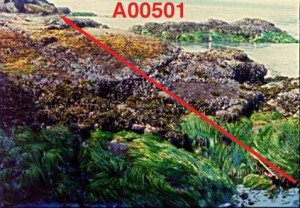
We have developed an exercise that allows one to take images from the transect file on the internet and process them, using the computer in order to quantify the ecological niche of organisms. The example provided is from the intertidal transect files from The Race Rocks ecological reserve, in Southern Vancouver Island, Canada.
Follow through the steps as indicated below.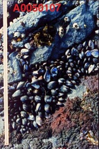 .
.
1. For instance from this image from the first transect, A00501, (A0 being the Race Rocks location, 05 being the sample station location and 01 being the first transect at that location, 07 being the seventh quadrat from the top of the intertidal zone. ). Quadrat 07 looks like this. By clicking on this icon you will see this one sample of the actual photo from the transect file.
2. If we want to define the space that the mussels occupy in this quadrat, we have to measure the percent of the quadrat that they are covering. This could be done simply by cutting out a piece of acetate that has been made by xeroxing a piece of graph paper and overlaying it on the screen.
3. A more precise way of doing this is by using an Imaging program to help analyse different aspects of the photograph. Download this image by clicking on the full size image then pressing and holding the right mouse button on a PC or pressing and holding the mouse of a Macintosh . Note that the mussels occupy a portion of this quadrat, a meter stick on the left side gives you the size of the quadrat.
4. CONVERTING THE IMAGES:
Since the above image is in a .JPG format , it has to be converted to a .PICT format for image processing. Do this with a graphic processing program .
5. Using GifConverter: Open the .jpg file obove that you have downloaded. Save it as a .PICT file. This is the format that is necessary to use in the next stage of the process, using NIH Image to measure features of the picture.
6. If you do not have a copy of the freeware NIH IMAGE. Download it from this site. (Both Mac and PC versions are available)
7. INSTRUCTIONS FOR NIH IMAGE: See this file :
Measurement of Surface Area Using “NIH IMAGE”
Also there may now be other software that is easier to use for measuring surface area coverage if one does a google search.
UPDATE: Also from NIH .. ImageJ. http://wsr.imagej.net/distros/
Calibration:
a) To calibrate the image in terms of real units: Use the straight line tool on the left panel, and draw it the length of the meter stick.
b) Use the pull-down menu called “Analyze”; go to “Set scale” . Change the units to centimeters, and “known distance” to 100.00, then hit “OK”.
c) To compute area: From “Tools” menu, select the heart-shaped tool. Outline the total area occupied by mussels. Click on “Analyze options” ; be sure the area box is selected). Press “OK”. From tool bar, select “Analyze”, “Measure”, “Analyze”, “Show results”. A table appears with the area of mussel coverage (in cm2). To compute % area occupied by mussels, measure the total quadrat area with the above procedure except use the rectangle measurement tool to outline the entire quadrat box.
8. DOWNLOADING THE TRANSECT IMAGES: Now, repeat this procedure with all the quadrats in the belt transect strip that contain mussels, you will also have to copy down the elevation found at the base of each quadrat as well..
Go to one of the transect files.
See Transect A0050101
See Transect A0050102
See Transect A0050103
9. Select one of the transects, and download the clips.
 10. USING A SPREADSHEET
Now we have to enter the data into an EXCEL or other suitable spreadsheet.. We will give the detailed instructions for EXCEL.
Enter data in column format (each column is a separate variable).
Calculate:
(a) % area covered by mussels for each transect (area covered by mussels/total area)
(b) percent slope: distance in perpendicular height (elevation change between adjacent quadrats divided by the linear distance (one meter) .
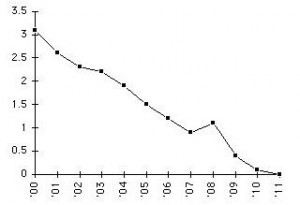
To evaluate terrain gradient for each transect (that is, the steepness of the intertidal shoreline), you can graph the relationship between elevation and slope .
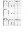 See this example .Here is a sample of the mussel distribution data as it appears on this spread sheet
 PLOTTING IN 3D
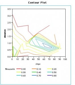
The goal of the analysis is to both describe and predict the environmental space that mussels must occupy in order to survive. The first step in the formal process is a graphical description of the environmental space actually occupied by the animals. In this example, the environmental space is the two dimensional space defined by the variables elevation and slope; the biotic “response” is the percent area occupied by mussels.We imported the variables X1 = “elevation”, X2 = “slope”, Y = “% mussel area” into a standard 3D graphics package (e.g. JMP-Contour Plot). The resulting graph gives the contour plots of mussel density as a function of the 2 environmental variables. Interpretation is similar to reading contour lines on an ordinary topographical map. Note that the “optimum” area for mussel settlement is a range of values for elevation and slope rather than a single point.
This file on Ecological Niche Models was developed by Penny Reynolds, Richard Rosecrance and Garry Fletcher at the Bioquest Consortium Workshop, on WHAT CAN WE LEARN FROM CONTEMPORARY MATHEMATICS REFORM? June 21-29, 1997. Beloit, Wisconsin. It was supported by a grant from the Howard Hughes Medical Institute to : The BioQuest Curriculum Consortium
1. Other websites on Photo transects :
Getting to the bottom of things
http://sango.churashima.okinawa/monitoring_en/cpc.html
 Return to the Contents page for Environmental modelling with Transects..
