BACKGROUND:
 Environmental abiotic and biotic factors can also be termed “Limiting Factors.“ They are limiting in that they tend to select only for those organisms which have the best tolerance, or adaptation to the factor. At different times of the year, some abiotic factors take on more importance than others. Water is certainly not a limiting factor at Race Rocks in the months of December and January compared to the dry months of July and August. In this assignment, we will examine data records and determine what other factors are variable in their importance in various times of the year. This assignment is paired with the assignment on Abiotic Factors
Objectives:
1. Present an argument for what you consider to be the most important abiotic factor in determining the distributions of organisms at Race Rocks , and contrast this with what you consider to be the most important factor in determining the distribution of organisms where you live.
2. Use the following terms to explain with graphs, examples of the concept of Limiting Factors.
- Euryhaline and Stenohaline
- Eurythermal and Stenothermal
3. Describe how Natural Selection of species occurs as the result of Limiting Factors.
4. Demonstrate how Limiting Factors of the environment determine and define the ecological niche of an organism.
5. Produce a graph demonstrating the Ecological Niche of an organism.
6. Discuss how our built up environments with cats, lawns, and other introduced species limit the ecological niches available and thus impact negatively on Biodiversity.
PROCEDURE:
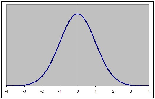
1.Introduction: Examine this graph representing the Normal Curve or a Bell Curve of the level of population of a species, in a certain area, or the density. If you think of the blue line here representing the number of individuals of animals or plants in a population, which exist in an environment with abiotic conditions favoring those at the central value of 0, then you can see that there is actually more positive selection for the central area being exerted than for either of the extremes. Species evolve in much this way. Those having the right amount of insulation, the right amount of ability to survive dessication or drying up, the right abilities to survive in a certain salinity or level of dissolved oxygen, or the right ability to tolerate a high level of wind in their environment, are the ones who are more successful in reproducing and thus their traits get passed along to more offspring. So the X-axis can represent the abiotic variables in an environment.
2. Correlate the month of occurrence of a species and the population levels for that month.
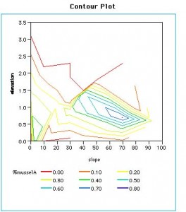
3. We can see from the assignment on abiotic factors, that there may be dozens of such graphs you could make for any organism.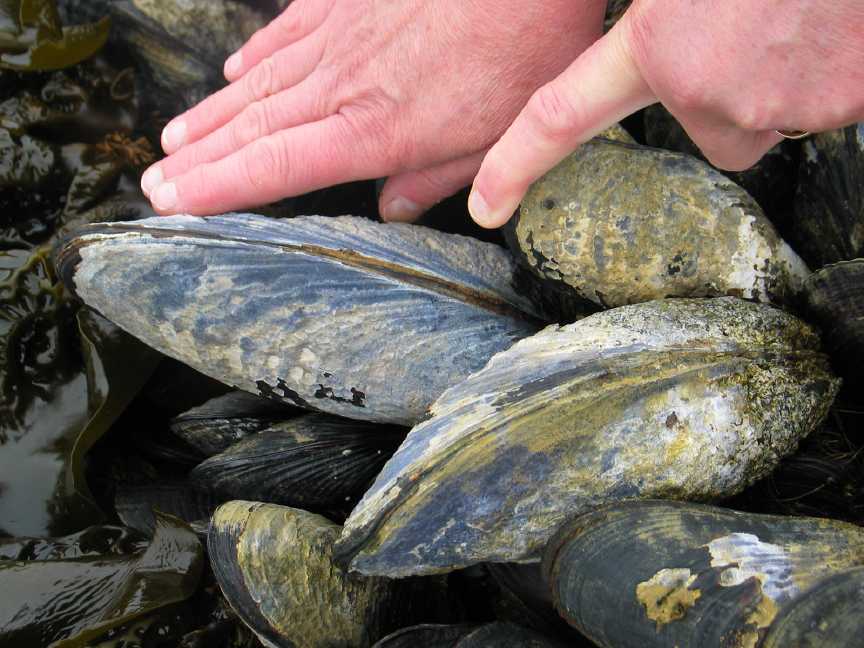 At Race Rocks, we have two species of the molluscs called mussels. They are Mytilus californianus and Mytilus trossulus . Visualize the x-axis above being a scale of temperature, for a marine animal such as a mussel, lets say the ideal temperature for mussels is 10 degrees C. Draw a similar graph with 10 in place of the 0 . Show the scale going up and down from 10. Lets say that the Mytilus californianus mussels cannot reproduce at a temperature higher than 12 degrees nor lower than 8 degrees C, so the blue line tapers down and ends at 8 degrees C. At Race Rocks, we have two species of the molluscs called mussels. They are Mytilus californianus and Mytilus trossulus . Visualize the x-axis above being a scale of temperature, for a marine animal such as a mussel, lets say the ideal temperature for mussels is 10 degrees C. Draw a similar graph with 10 in place of the 0 . Show the scale going up and down from 10. Lets say that the Mytilus californianus mussels cannot reproduce at a temperature higher than 12 degrees nor lower than 8 degrees C, so the blue line tapers down and ends at 8 degrees C. |
4. Now plot another graph on the same scale, This one is for the other local mussel, Mytilus trossulus. 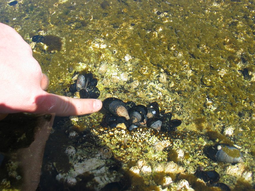 It lives in the intermediate level tidepools and can survive in water up to 16 degrees and down to 4 degrees. In the sample above we say that the M.californianus is a Stenothermal ( narrow range of tolerance to heat) animal, whereas the M.trossulus is a Eurythermal (wide range of tolerance to heat) organism It lives in the intermediate level tidepools and can survive in water up to 16 degrees and down to 4 degrees. In the sample above we say that the M.californianus is a Stenothermal ( narrow range of tolerance to heat) animal, whereas the M.trossulus is a Eurythermal (wide range of tolerance to heat) organism |
| 5. Next we will do a similar plot for salinity. Here 30 parts per thousand for salinity becomes the central measurement and above and below that amount make the rest of the scale. M.Californianus prefers to live in water that is 27 parts per thousand. But it can live in up to 30 or down to 25. M.trossulus also prefers 27 parts per thousand, but can live in water that ranges from 32 down to 22 parts per thousand. Now if we combine the same prefixes: Eury and Steno,with the word haline, we will get a word that describes the organisms. So now you have two new words that help describe the variation the same abiotic factor can have on two closely related species. |
6. Natural Selection which can lead to the evolution of separate species, is often determined by the way an organism is able to tolerate variations in the abiotic factors of it’s environment.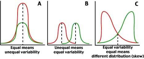 Just when that seemed so straightforward, we have to recognize that selection pressure may affect the same species group in different ways. Two species of mussel may on the other hand prefer different ranges of temperature or salinty instead of the 10 degrees. The picture B could represent that situation. What would the skewed distribution in C therefore represent in terms of selective pressures on the population? Just when that seemed so straightforward, we have to recognize that selection pressure may affect the same species group in different ways. Two species of mussel may on the other hand prefer different ranges of temperature or salinty instead of the 10 degrees. The picture B could represent that situation. What would the skewed distribution in C therefore represent in terms of selective pressures on the population?
9. Extension Materials: Central Tendency and Variability Also, you may wish to take this opportunity to get into an exercise on Standard Deviation. To draw such a curve as the Normal Curve at the top of the page, one needs to specify two parameters, the mean and the standard deviation. The graph has a mean of zero and a standard deviation of 1, i.e., (m=0, s=1). A Normal distribution with a mean of zero and a standard deviation of 1 is also known as the Standard Normal Distribution. |