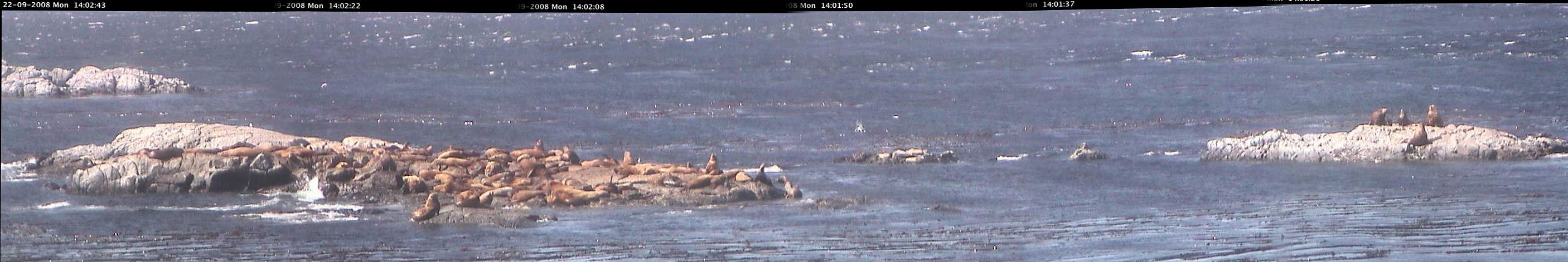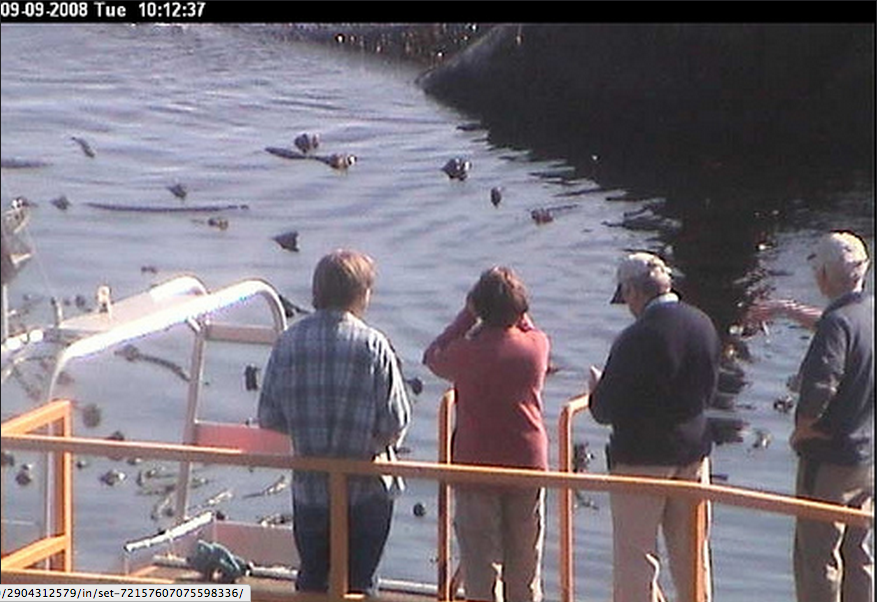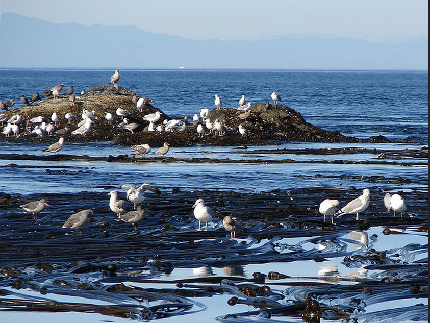
A visual census using the remote camera 5 focused on Middle Island.
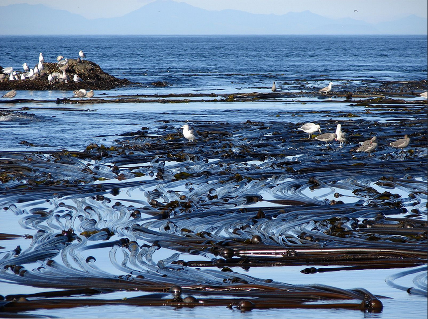
The following panorama was taken of the “middle islands” at Race Rocks from 6 images taken consecutively with a small overlap and then spliced together with a “Photostitch” program which is usually available with the software for an electronic camera.
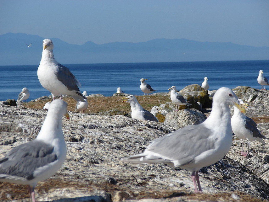
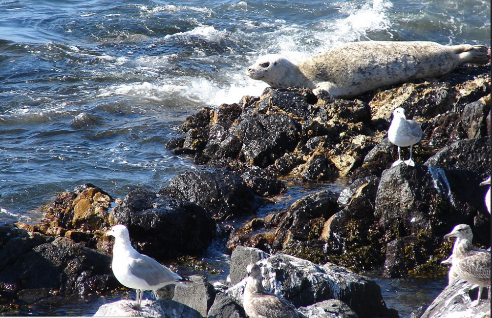
Educational Application: When we build up a set of these pictures, students can do mathematical projects by going on the camera and getting a live count and then running various statistical comparisons on these archived images. Just click on the image below for a version that is large enough to enable counting and identification.
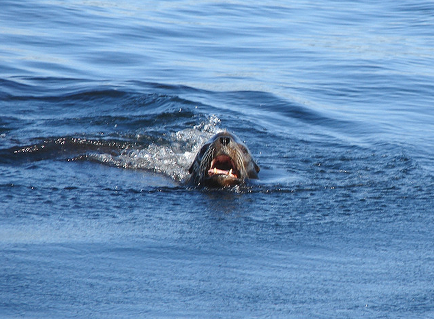
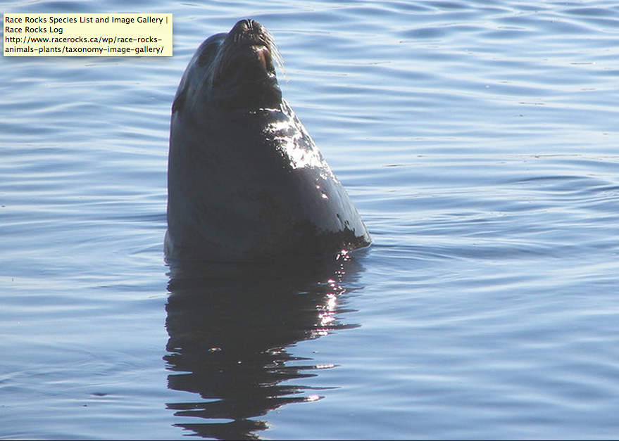
Click for larger size to count sealions.