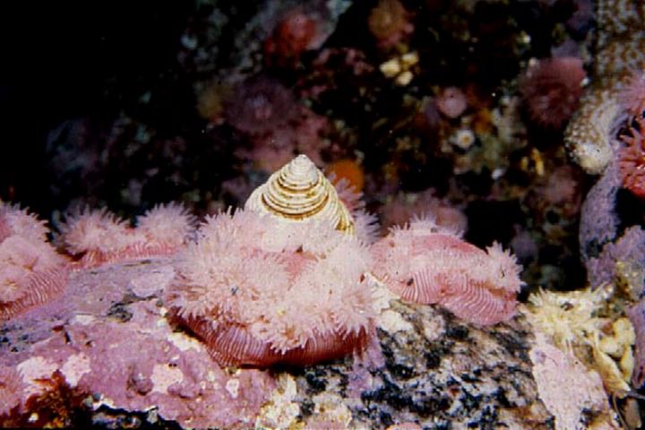
Conical shell usually orange-yellow, dotted with brown and with a bright purple or violet band encircling the lower edge of each whorl, with 8 or 9 whorls; body of living animal orange, with brown dorsal spots. Size to 30 mm height.
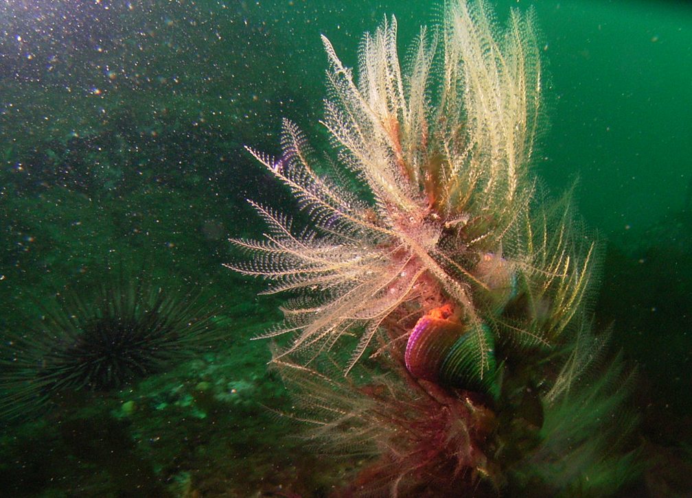
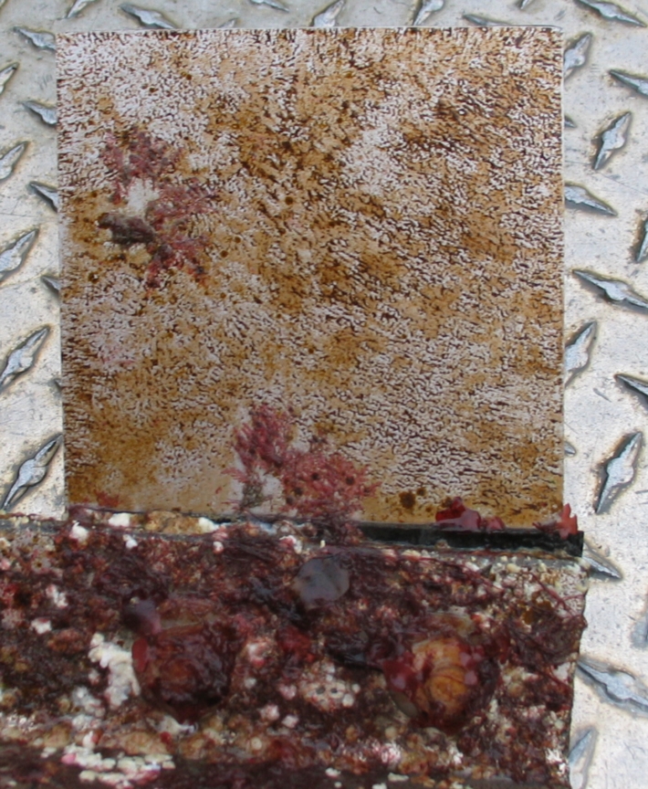
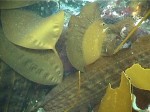
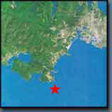
Range: Alaska south to Baja California. They occur very rarely at Race Rocks. They are more common however on the islands to the West, Church Island and the Bedfords in Beecher bay, and as in the photo below , Secretary Island, outside of Sooke harbour.
Unicode
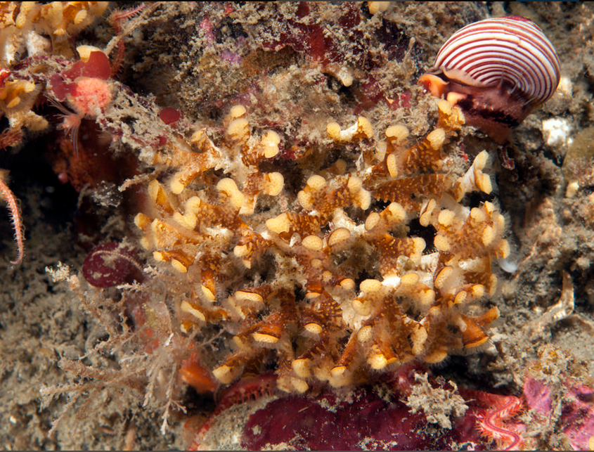
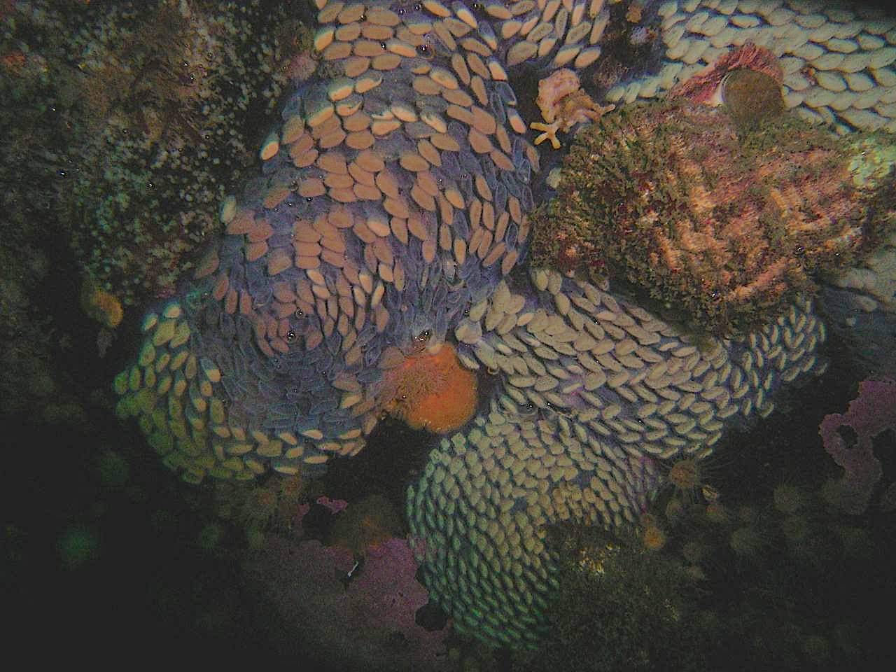
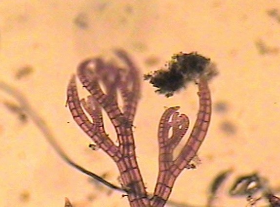
This photo was taken on Secretary Island, several kilometres west of Race Rocks where this species occurs more frequently than at Race Rocks. Chris Blondeau captured the snail grazing on a clump of Plumularia hydroid.
Conical shell usually orange-yellow, dotted with brown and with a bright purple or violet band encircling the lower edge of each whorl, with 8 or 9 whorls; body of living animal orange, with brown dorsal spots. Size to 30 mm height.
Range: Alaska south to Baja California. They occur very rarely at Race Rocks. They are more common however on the islands to the West, Church Island and the Bedfords in Beecher bay,and as in the above photo, Secretary Island , outside of Sooke harbour.
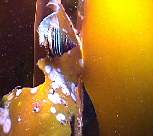
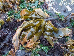
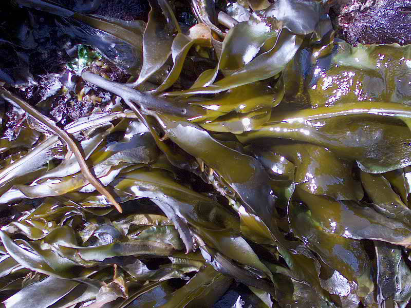
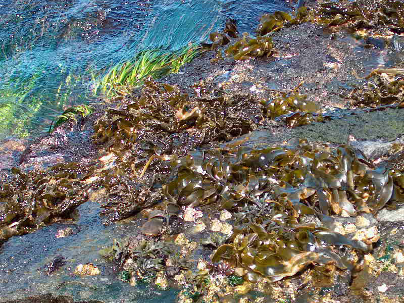
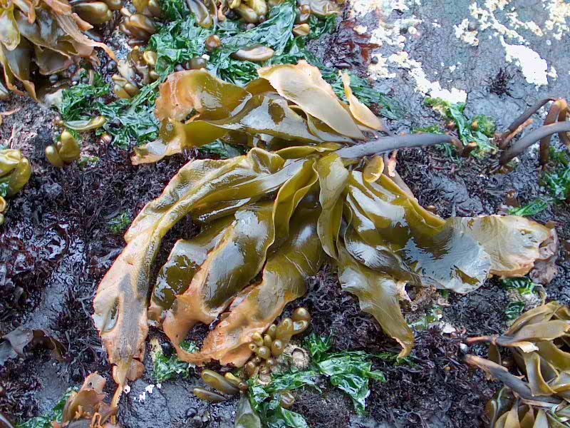
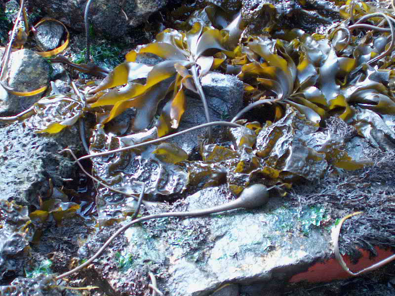
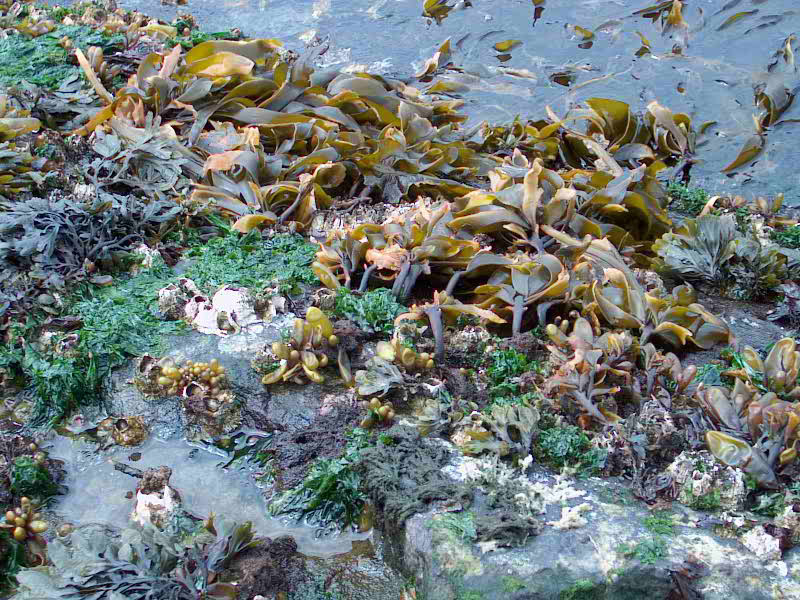
Habitat: on the open coast. Calliostoma annulatum reportedly moves up the kelp stipes to near the sea surface in ‘bright weather’ and descends under other conditions. These animals can move rapidly.
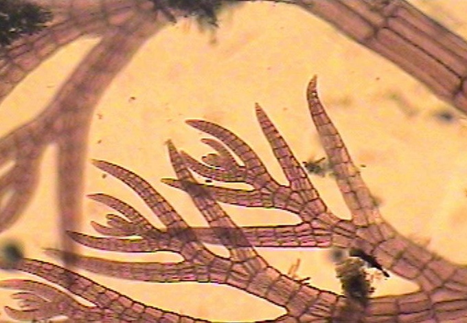
It’s an omnivore. In the spring the food is mainly the kelp itself; the snail prefers animal foods when these are available especially hydroids (e.g. Obelia sertularians) and encrusting bryozoans (Membranipora; Hippothoa), Detritus and some diatoms and copepods are taken, too.On the sea floor, they take some of the cnidarian Corynactis californica and scavenge on dead fish. In aquaria, the snails have been seen to eat hydroids, the anemone Epiactis prolifera, the stalked jellyfish Haliclystis, dead nudibranchs (Polycera atra), dead keyhole limpets (Diadora ), dead chitons, nudibranchs eggs, and other items, including even canned dog food. Although jaws are often poorly developed in the Trochidae, observations by Paron (1975) suggest that they play an important role here. Hydroids stems in the gut often appeared ‘neatly cut into short segments’. Further when attacking anemones, Calliostoma annulatum after initial contact, ‘would rear up on its metapodium, expand its lips, and suddenly lunge forward while bitting at one of the anemone’s tentacles. A dorid nudibranch was also attacked in this way.
The shell bears a layer of mucus which makes it slippery and not easily held by potential predators.
Reproduction: Males usually spawn first. Green eggs, each in clear envelopess and a gelatinous coat thick, are shed in a soft gelatinous coating. In the San Juan Archipelago, specimens collected June-August may spawn if placed in sea water at 18-22 C
Domain Eukarya
Kingdom Animalia
Phylum Mollusca
Class Gastropoda
Subclass Prosobranchia
Order Archaeogastropoda
Superfamily Trochacea
Family Trochidae
Genus Calliostoma
Species
annulatum
Common Name: Top snail or Top shell
References:
Harbo, R. 1997. Shells & Shellfish of the Pacific Northwest -A field guide.- -Pg. 75-. Harbour Publishing.
Kozloff, E. N. 1996. Marine Invertebrates of the Pacific Northwest Coast -Pg. 203-. University of Washington.
Morris, R.H., Abbott, D, and Haderlie. 1980. Intertididal Invertebrates of California. -Pg. 250-. Stanford University Press, Stanford California.
Strathmann, M. 1987. Reproduction and Development of Marine Invertebrates of the Northern Pacific Coast. Data and Methods for the Study of Eggs, Embryos, and Larvae. -Pg. 233-234-. University of Washington Press.
Other Members of the Phylum Mollusca at Race Rocks.
 Return to the Race Rocks Taxonomy Return to the Race Rocks Taxonomyand Image File |
 The Race Rocks taxonomy is a collaborative venture originally started with the Biology and Environmental Systems students of Lester Pearson College UWC. It now also has contributions added by Faculty, Staff, Volunteers and Observers on the remote control webcams. The Race Rocks taxonomy is a collaborative venture originally started with the Biology and Environmental Systems students of Lester Pearson College UWC. It now also has contributions added by Faculty, Staff, Volunteers and Observers on the remote control webcams. |
Feb. 2002 Maria Belen Seara PC yr 28

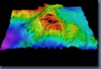 The small, rocky outcrops are home to seals, sea lions, elephant seals and birds, as well as the buildings and equipment of the Race Rocks Lighthouse. These outcrops are literally the tip of the ecosystem New leading-edge bathymetry reveals Race Rocks as a giant underwater mountain. The diversity of marine life is breathtaking and still not fully explored. The teachings of Salish elders merge with more recent science to explain the mysteries of nature at Race Rocks.