Measurement of Surface Area Using “NIH IMAGE”

Posted on Tuesday,April 15, 2003 by Garry Fletcher

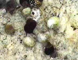
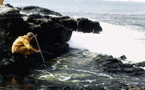
The image that you have available must be either a .Tiff or a .Pict . You may download the full screen version of this image, pool5.jpg and then convert it to one of those formats using graphics converter or Photoshop or any suitable image handling program.The image of the tide pool shown here has a 1 meter ruler in it . An object of known length must be present in the picture in order to do measurements.

1. Open NIH image using the small black microscope icon. (If you do not have NIH Image installed on your computer you may download it here. download NIH Image ( available in Mac or PC)

2. Open the image “pool5.pict” that you have made by downloading the “pool5.jpg”.

3. From the TOOLS pop-up menu in NIH Image, select the SELECT LINES tool ( the dotted line fifth from the top of the right hand column).

4. Click and drag the select lines tool over the one meter image in the picture.

5. Click on the top Menu bar item ANALYZE, then move down to SET SCALE

6. In the SET SCALE box, set the units to centimeters. Set the KNOWN DISTANCE to 100., press “OK“

7. Select the region to measure using the freehand selection tool, ( fourth down on the Tools bar– heart shaped dotted line.)

8. Outline the area to be measured by tracing the perimeter of it with this tool.

9. CLICK on ANALYZE– OPTIONS – in the tool bar.

10 .Click in the boxes for Perimeter and Area. ( Other options may be tried after this basic step has been mastered.)

11. Click on ANALYZE — MEASURE –ANALYZE–SHOW RESULTS . Now you should see the calculated area and perimeter in the results box.

Further information on page 6 of the “NIH Image” direction manual

Surge Channel and Surge as an Abiotic factor

Posted on Tuesday,April 15, 2003 by Garry Fletcher

On a field trip to Race Rocks with the Biology class in the spring 2003, we took some time to observe and video the surge channel out on the south-west tip of Great Race Rock. It was a calm day which had been preceded by a few days with storms out in the Pacific Ocean. The energy imparted to the water column was just now reaching Great Race and the water was breaking on the west shore. The effect of “Surge” as an abiotic factor is not often considered in affecting the intertidal zonation of organisms on rocky coastlines in marine biological research. See this file on this abiotic factor.

It is our firm belief that here, the level up the shoreline in the intertidal zone where many invertebrates and algae can survive is elevated. These intertidal organisms are able to keep moistened longer, ambient temperatures are depressed from evaporation and and they even have longer availability to food resources being carried in the surging water. This is most obvious with the Goose Neck barnacle population and the intertidal anemone distribution along this shore. Additionally the tidepools up the channel are flooded more frequently, resulting in lower temperatures and more stabilized salinity conditions. It should be emphasized that this is not directly “wind-driven” water movement. As one can see in the video, the surrounding sea is calm, with little wind that day.

Tidepool Studies at Race Rocks Pool #4 Peg6

Posted on Tuesday,April 15, 2003 by Garry Fletcher

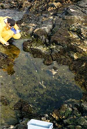
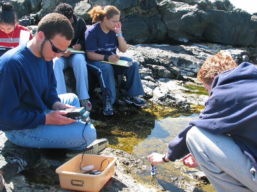
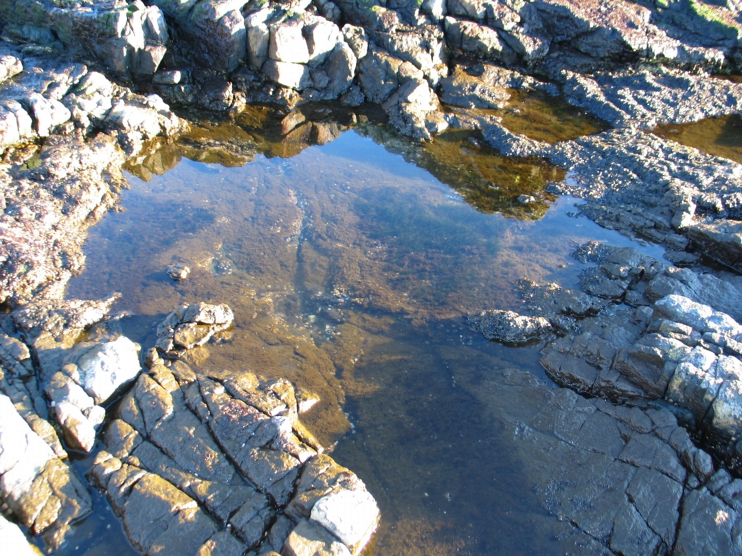
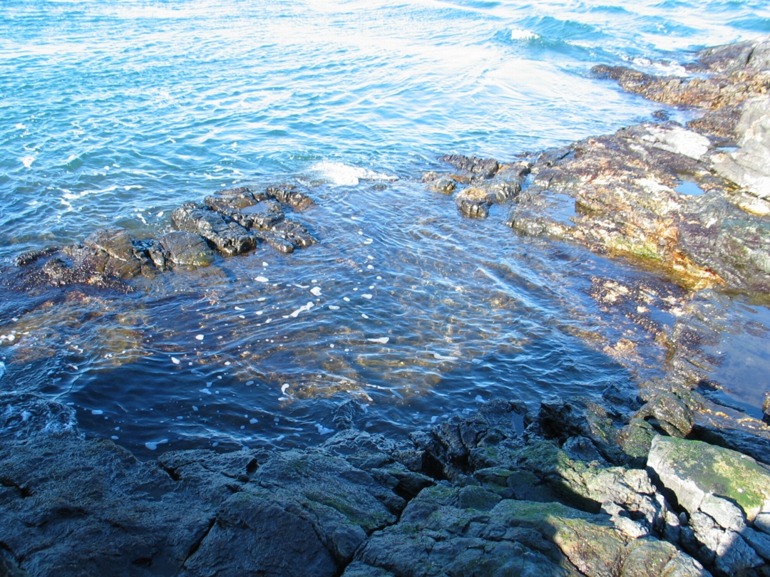
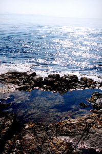
A general view of the pool.It is perched on a shelf which easily gets flooded when there is a slight swell in the ocean.	Polymorphism in the Snails of Pool # 4, Extended essay in Environmental Systems,
A student examines the life of pool 4	Amphipods collected with a suction bottle from pool#4.
A microscopic picture of the diatoms that grow as a fuzz in the pool in the early spring. They remain a few months until they are grazed off.	Roberto and the Biology Class measure salinity in pool 4.. May 2004
Enteromorpha growing in the pool. May 2004.	Bay mussels, Mytilus trossulus in the brackish water of Pool#4
In May 2004,it is clear where the grazers, Littorina snails and amphipods) have trimmed off the diatoms on the bottom.	Arunas measures the depth of pool 4 while watching for swells
In February, 2007, the diatoms cover almost the entire bottom of the pool. This is the winter pattern. Grazing as shown above gradually removes the covering of diatoms.	January, 2007. The tide is at its peak today, showing pool 4 being entirely submerged.
On February 11, 2008 a beast is photographed in the tidepool.	Close up of the Filamentous golden algae filling the tidepools in early spring.
Weird form shades a covering of diatom fuzz!

Some ideas to consider:

Invitations to Inquiry:

This pool is unique in a number of ways. The white substrate in the bottom of the pool is the result of a quartz intrusion that has flooded while molten, through the cracks of the basalt.
What is the effect of this white reflective surface on the temperature of the pool and the organisms that live in the pool?

In 1997 while doing a detailed analysis of the organisms in the pool, we noticed for the first time that there were white periwinkles. At that time 26 were counted by Nadia and Catherine. Speculate on the evolutionary implications here.

The mussels in pool #4 are Mytilus trossulus, the bay mussel. Mussels that you can see on the surrounding intertidal areas are the Mytilus californianis. Why the species difference?

The pattern of diatom distribution changes in the bottom of the pool. In the winter, it covers the pool with a thick felt-like appearance, as spring approaches, the cover of diatoms starts to disappear, starting along the cracks where the mussels are anchored.. could one measure the rate of grazing from the amphipods in the cracks?

Temperature and Salinity in the pool fluctuate widely and at times form stratified layers. How does this affect organism distribution.?

The biotic and abiotic features of this pool vary considerably from other pools in the near vicinity. Quantify and explain the differences or similarities.

The only other pool that resembles this one is found over on the north-east corner of the island, at location peg15-pool #14. Compare the biotic and abiotic factors of these two pools, and explain the differences.

The following lab on tidepool abiotic factor measurement was done by Chiara Ravetti in September,2005.
Biology Laboratory

Analysis of the Abiotic Factors in Race Rocks Tidepools

The measurements of salinity, ph, and temperatures of different tidepools at Race Rocks was done September19, after 11.30 a.m., with high tide. For this reason the pools selected were only five, two (pool 7 and 8) several meters away from the sea at that time of the day, the other three (pool 1, 2 and 4) closer to the water and larger.
Data analysis and further note

	pool 1	pool 2	pool 4	pool 7	pool 8	Ocean water
Salinity	62.1	32.8	21.9	45.3	45	30
Temperature	14.4 C	14.4	14.2	15.4	15.2	10
ph	8	6.8	6.9	7	8	—

The measurement of salinity is expressed in parts per thousand; the instrument utilizes electricity, that passing through salt ions determines its quantity.
The pools were contaminated by sealions excrement, which reduced the visibility inside the pool and probably altered the pH of the water.
Other factors which might affect these values in a tidepool are: evaporation, precipitation, and in general pollution, scarce precipitation at that time of the year, the presence of the estuary, (The Strait of Juan de Fuca) with the influence of fresh water. The salinity in a tidepool is higher than the sea, for the evaporation and the little exchange of water, therefore the organisms living in it must tolerate high salinity, as well as variations in temperature. The smaller tidepools further from the sea present even more significant changes.

Carmen’s lab on Transects

Posted on Tuesday,April 15, 2003 by Garry Fletcher

Race Rocks Transect Lab

Kite Diagrams

BELT TRANSECT PROCEDURE

About 20 meters from the dock on the north side of Great Race Rocks, we plotted our transect. Starting at the shore and going 15 m inland, we laid a tape measure and at every half-meter we made a 50cm-by-50cm quadrant and counted the species in the plot.

ANALYSIS: We counted the algae by percent cover and the invertebrates by number. Some species overlapped, such as anthopleura and halosaccion. This coexistence was possible because the two species were not vying for the same food source. Species such as thatched barnacles and acorn barnacles did not live in the same quadrants, however. This may be because they are competing for the same substrate and nutrients and each prevents the other from invading into their space. As well, the thatched barnacles stopped growing at quadrant 15 but that is just where its competition, acorn barnacles began to grow. Perhaps one species was better suited to surviving farther up the shore.

That was the case for many of the species along the transect. Invertebrates like chiton, limpets and snails needed to be covered by the tide for most of its cycle. If these species tried to grow where they were exposed for a longer period of time, they would dry out and die. Other species like lichen need to be out of the water and as expected, were only found at high elevations on the transect.

The topography also affected the species diversity. The California Mussel, for example, was found only in quadrants that had crevices and rough substrate on which to grow.

In general, the abiotic factor that had the greatest affect on species diversity on the transect was the elevation and amount of tide cover the area got during a tide cycle. Below are kite diagrams of each species we found on the transect.

Carmen and Jana Environmental Systems class April 2003

LINK to photographic transect strip of this area

This x-axis represents percentage cover for the macroalgaes. Note it may be a different scale in the graphs. The y-axis represents the .5meter quadrat location from the peg #15.

The “series” 1 and 2 just represent half of the value for each quadrat for the species, a way to get EXCEL to plot a symmetrical “kite” shape