Myxilla incrustans: incrusting sponge– The Race Rocks Taxonomy

This sponge can be found on rocky subtidal areas at Race ROcks  It commonly grows over the surface of swimming scallop shells. It is believed to form a mutualistic association with the swimming scallop, obtaining a moveable substrate while preventing predation of the scallop. Apparently the smell of the sponge deters the sea stars which may be intending to prey on the scallop

crustsponge

The volcano-like oscules on the sponge which is attached to the valve of a swimming scallop.

ah052010scallopl

Adam harding took this photo off the docks at Race Rocks. The shell of the scallop is covered with the orangish layer of sponge with attached hydroids.

It is an extremely variable widely distributed species ranging from intertidal to 2540 m
Colour: the colour in life ranges through various shades of gold occasionally to a light gold-brown with a slight tinge of rose. In alcohol the sponge is grey-white to yellowish-brown.
Form: The sponge is incrusting or occasionally massive
Size: Intertidal incrusting forms re up to 8 cm thick an 20 cm in diameter. Dredged massive forms have a diameter of up to 9 cm. Fistules are up to 25 mm high.
Consistency: the consistency is moderately firm and tough. some specimens are weakly spongy and fragile.
Surface: The surface varies from slightly roughened and tuberculate to highly rugose and fistulated. It is somewhat rough to the touch
Oscules: oscules are common or abundant and irregularly distributed. Oscules may be elevated on fistules when the latter are present. Oscules are from 033 to 8 mm in diameter.
Pores: pores are abundant and measure from 20 to 270u in diameter.


rmincrustingsponge

Detailed view of the incrusting sponge on a swimming scallop

rmincrusting

Ryan Murphy took this image of the various colours of the sponge

Domain Eukarya
Kingdom Animalia
Phylum Porifera
Class Demospongiae
Order Poecilosclerida
Family Myxillidae
Genus Myxilla
Species incrustans
Common Name: incrusting sponge


This file is provided as part of a collaborative effort by the students of Lester B. Pearson College
Oct 2003 Roberto Ruglio year 30

Phalacrocorax pelagicus: Pelagic cormorant–The Race Rocks Taxonomy

rmpelagichorm

Pelagic Cormorant,  Phalacrocorax pelagicus photo by Ryan Murphy, 2010

See images of Pelagic Cormorants on Ryan Murphy’s Flickr site

Range of the Pelagic Cormorant:
Breeds from the Bering Sea to Japan and south to near San Diego, USA.  Winters in the Aleutian Islands and along the coast from British Columbia to Baja, California.

Pelagic cormorants nest at Race Rocks and live there year-round. They prefer the cliff to the West of the camera 5, and can often be seen perched there along the cliff edge (picture above left)

Nest:
The nest is a mass of seaweed and grass on a cliff.  Pelagic cormorants nest in colonies and like ledges so narrow they must land and take off facing the cliff. During the years between 1980 and 1995 numbers of nests ranged above 20. In the years 2000, 2001,2002 there was complete nest failure due to the lack of herring feed in the surrounding waters. During 2003 , 2004, and 2005 only two or three nests have been established with successful hatches.

Following  are pictures taken in the nesting season by G.Fletcher in the 1980s and 1990’s when there were pelagic cormorants nesting at Race Rocks:

Local Numbers of Phalacrocorax pelagicus
Xmas bird count

Screen Shot 2014-12-20 at 8.06.55 PM

Pelagic Cormorants–Ryan Murphy photo

Year
1997–14
1998–2
1999–20
2000–14
2001–12
2002–20
2003- no census taken..too stormy!
2004- 110

rmpelagiccorm22010

Pelagic Cormorant–Ryan Murphy photo


2005- 20
2006-20
2007-42
2008-storm
2009-90
2010-78
2011-0
2012-0
2013-17
2014—

rmpelagiccorm2010

Pelagic Cormorant–Ryan Murphy photo-2010

Classification:
Domain: Eukarya
Kingdom: Animalia
Phylum: Chordata
Class: Aves
Order: Pelicaniformes
Family: Phalacrocoracidae
Genus: Phalacrocorax
Species: pelagicus
Common Name: Pelagic cormorant


We have seen a marked decline in nesting of one of the four species of seabirds which has nested traditionally at Race Rocks, Pelagic Cormorants (Phalacrocorax pelagicus). By 2007, the nesting population had been reduced to one or two nests, and from 2008 to the last season (2009 ) there were no nests at all. This population crash has been common across the Gulf Islands., and the lower end of Vancouver Island and Strait of Juan de Fuca. According to the Canadian Wildlife Service, the population of this species is estimated to be at 9000 individuals, and the pelagicus subspecies is red-listed by BC – other subspecies are stable.

RM_males-and_female_pelagic_cormornat

Two males and a female pelagic cormorant

In this attached file, I have summarized the results of several papers on research on Cormorant populations in the southern Gulf Islands and Georgia Strait. Vermeer and Rankin, 1984, did their research when the populations were on the incline, however since the 1900s, this trend has not persisted as has been reflected in the paper by Chatwin et al. The summary of their paper and the possible reasons for decline are listed near the end of this review.

See other posts of Pelagic Cormorants at Race Rock

taxonomyiconReturn to the Race Rocks Taxonomy and Image File
pearsonlogo2_f2The Race Rocks taxonomy is a collaborative venture originally started with the Biology and Environmental Systems students of Lester Pearson College UWC. It now also has contributions added by Faculty, Staff, Volunteers and Observers on the remote control webcams. Garry Fletcher, 2003


Arctonoe vittata: Commensal scale worm–The Race Rocks Taxonomy

scaleworm

Scaleworm on the striped sunstar.( from video)

Physical description

The Arctonoe vittata (formerly known as Halosydna lordi) usually have around 25 or more pairs of scale, which they sometimes shed when they are disturbed. Arctonoe grows up to 8cm to 10 cm long and is usually light yellow. However the color may change depending on its host. Scientists do not know wether this is due to a certain compound on the host that changes their color, or wether it is because they basically eat the same thing, but the scale worm usually very lightly changes its color according to its host.

Distribution in the world: Scale worms live in the North Pacific ocean. It is one of the most studied worms and it has been mostly studied near the coasts of Japan and also near Kamtchaka, far east Russia. It also lives in the north west coast of North America, including the coast of British Columbia. It lives mostly in salt water and almost never in fresh water.

Biotic Associations: The Arctonoe vittata a commensal worm, lives on other species. It observes a positive relationship with its host, notably the starfish Asterias amurensis or the mollusc keyhole limpet Diadora aspera It usually lives near the oral part of its host, and when there are two A.vittata there, the other one will live on the arm if it is living on a starfish. The length of the worm is big considering the size of its host, sometimes its ends almost touch when it is curled up on the oral orifice. It mostly likes to live on larger hosts because they are older and more exposed to plankton. If the A.vittata is living on the keyhole limpet, and the keyhole gets attacked by a starfish, the worm will sense that the demise of its host will lead to its own demise. Thus it will bite the seastar’s tube feet and cause it to withdraw. The scale worm is attracted to chemicals released by it’s host. It is interesting to note that the host is also attracted by chemicals released by the commensal worm. The commensal worms seemed to have a different taste for their host depending on which part of the world they came from. However, the limpet Acmaea pallida was the overall favorite host.

Interesting local behavior: Some scale worms have been spotted on seastars. They were colored white, the same as the underside of the star. There have also been some scale worms spotted on sea cucumbers, they were of a reddish color, and were the Red commensal scale worm Arctonoe pulchra

Reproduction and feeding: The A.vittata bites off the food that is left over from the side of the mouth of its host. They are usually fatter if they are located near the mouth of the host. The worms are hermaphrodites. The worm will leave eggs on its host, some grow there, usually the first ones. The rest will move to a different host because there is too much competition with the one that is already there.

Domain Eukarya
Kingdom Animalia
Phylum Annelida
Class Polychaeta
Order polychaetes
Family polynoidae
Genus Arctonoe
Species vittata

Other Annelids at Race Rocks

taxonomyiconReturn to the Race Rocks Taxonomy and Image File
pearsonlogo2_f2The Race Rocks taxonomy is a collaborative venture originally started with the Biology and Environmental Systems students of Lester Pearson College UWC. It now also has contributions added by Faculty, Staff, Volunteers and Observers on the remote control webcams.  Oct 2003, Lindsay Cheong

with underwater photography of Ryan Murphy

Notoplana acticola: flatworm– The Race Rocks taxonomy

Notoplana acticola is a polyclad flatworm and it is one of the common polyclads of rocky shores. A specimen may be more than 2cm in length, but the average is about 1cm. We find these occasionally in the mussel beds and under rocks in the lower intertidal.

notoplanaacticola

Some mature Notoplana acticola are sometimes found as hermaphrodites.

Notoplana acticola lives in the upper tide pools and it may be abundant in the lower tide pools as well.

Domain Eukarya
Kingdom animalia
Phylum platyhelminthes
Class turbellaria
Order polycladida
Family otocelid
Genus notoplana
Species  acticola
Common Name:  flatworm
This file is provided as part of a collaborative effort by the students, faculty, staff, and volunteers  of
Lester B. Pearson College

Oct 19, 2003
Aline Celine

Tide Pool Abiotic factors

In the high intertidal areas of Race Rocks, there are tidepools with wide fluctuations of abiotic factors. The organisms inhabiting these pools are well adapted to these extremes. Garry talks to a biology class about some of the variables influencing these high tide pools, and the flagellated green algae living within them.

Racerocks.com Activity October, 2003

Race Rocks Ecological Reserve and the web activity. The racerocks.com activity went out to Race Rocks to practise live webcasting from the island.

Apodichtys flavidus: The Race Rocks Taxonomy

These images were taken on the remote camera 5 shows a Pigeon Guillemot prior to feeding a Penpoint gunnel to chicks.During the months of May and June, the Pigeon Guillemots (Cepphus columba) are constantly diving off the north side of Great Race Rock and bringing up penpoint gunnels for their young. They nest under loose rock on several locations arounf the island. They are very cautious about going to their nest burrow where they may be seen by predators,

PUGET SOUND/ Strait of Juan de Fuca SPECIES

Apodichthys flavidus Penpoint Gunnel

Pholis clemensi Longfin Gunnel

Pholis laeta Crescent Gunnel

Pholis ornata Saddleback Gunnel

Pholis schultzi Red Gunnel

Xererpes fucorum Rockweed Gunnel

PENPOINT GUNNEL

This is a family of littoral fishes of the northern Pacific and northern Atlantic.They are typically found hiding under rocks and logs or in tidepools at low tide.The longest gunnel , at maximum of 46 cm,is the Penpoint Gunnel.Most gunnels feed on small crustaceans and molluscs.There are about 14 species, six are found here. Although secretive , this family is common in Puget Sound. This fish is not important commercially and is not considered threatened.This species can breath air when out of water.

PHYSICAL DESCRIPTION: Body elongate and compressed (eel-like body with no pelvic fins). Contains only flexible spines ,may have a dark streak that runs through the eye from top of head downward . Eye round, its diameter about one fifth the into length length of head. It may have small dark spots along the sides.Distance from snout to anal origin greater than half of body length.Maximum length is 1.5 feet.10 large melanophores along dorsal surface of gut and anus, melanophores can be also along postanal and dorsal near caudal region,ventral surface of gut has a row of small melanophores.Colour very variable depending upon diet as well as environment, from green through brown to red, the green colour from pigments dispersed through skin, the red in special pigment cells, the brown in combination (Hart 1973).Teeth are sharp,pointed, apparent in post-larvae.

Dorsal fin KC-XCIV (Miller and Lea 1972).

Anal fin I,36-42 (Miller and Lea 1972); I,38-42 (Hart 1973).

Pectoral fin 15-16 (Hart 1973).

Mouth Terminal,small,with thick lips (Hart 1973).

Verebrae 96-101 (Miller and Lea 1972)

DISTRIBUTION: Southern California to southeast Alaska and Kodiak Island.In British Columbia on both coasts of Vancouver Island, the Strait of Georgia .Common in Burrard Inlet in September.Queen Charlotte Islands (Hart 1973). In costal or bay water blending with vegetation such as Sargassum spp.,Ulva spp., and Zostera spp.,settling on the bottom at ca. mm TL (Wilkie 1966).Pelagic,along coastal waters and bays. Horseshoe Cove and vicinity of Portero Power Plant on San Francisco Bay,Marconi Cove of Tomales Bay.

REPRODUCTION: Spawing occurs from January to March.The egg mass is coiled around by one or both parents.The incubation period is about two and two a half months.Newly hatched larvae average about 13mm, and the body is transparent and positively phototactic (Wilkie 1966).The age of maturity of the penpoint gunnel has not be documented in the literature.Growth appears to be rapid during the first year from 20 to 40 milimeters in April and May to 100 to 120 millimeters by the end of summer.

REFERENCES: J.L.Hart- Pacific Fishes of Canada(1973),Wilkie (1966)


taxonomyiconReturn to the Race Rocks Taxonomy
and Image File
pearsonlogo2_f2The Race Rocks taxonomy is a collaborative venture originally started with the Biology and Environmental Systems students of Lester Pearson College UWC. It now also has contributions added by Faculty, Staff, Volunteers and Observers on the remote control webcams.

March 8 2003- Miroslav Lestanin


Syllabus connections
to racerocks.com
Syllabus Details – Topic 4: Ecology and Evolution and OPTION G

4.1 Communities and Ecosystems (5h)
This reference is adapted from a Syllabus of the IB. In no way is it intended to replace parts of that syllabus, it is intended only to enhance your links with racerocks.CA references to such syllabus objectives . Only the Ecology -related topics are presented here.

The brown text
and the
blue hyperlinks
..take you to a file that presents Race Rocks data or reference material relating to the objective stated.
4.1.1 Define ecology, ecosystem, population, community, species and habitat. 1
    • Ecology—the study of relationships between living organisms and between organisms and their environment.
    • Ecosystem—a community and its abiotic environment.
    • Population—a group of organisms of the same species who live in the same area at the same time.
    • Community—a group of populations living and interacting with each other in an area.
    • Species—a group of organisms which can interbreed and produce fertile offspring.
    • Habitat—the environment in which a species normally lives or the location of a living organism.
Ecosystems on different scales are represented at Race Rocks. Structure and function can be studied using the assignments presented in the OceanQuest assignments Abiotic factors are available in the environmental data and sensors section.
4.1.2 Explain how the biosphere consists of interdependent and interrelated ecosystems.
.Internal Link:
Campbell Biology Images ( Internal link) Introduction to Ecology chapter 50
http://peernet.lbpc.ca/BIOLOGY/Campbell_Biology/imagelibrary/ImageLibrary40-55/50-EcologyAndTheBiosphere/HTML/index.html
3
4.1.3 Define autotroph (producer), heterotroph (consumer), detritivore and saprotroph (decomposer). 1
4.1.4 Describe what is meant by a food chain giving three examples, each with at least three linkages (four organisms).
note: In my opinion, the term food chain should never be used as it is misleading! (GF)
2
Food chains are best determined using real examples and information based on natural ecosytems. A -> B indicates that A is being “eaten” by B (ie the arrow indicates the direction of energy flow). Each food chain should include a producer and consumers, but not decomposers. Named organisms at either species or genus level should be used. Common species names can be used instead of binomial names.
4.1.5 Describe what is meant by a food web Internal Link:Campbell Biology Images ( Internal link) Ecosystems chapter 54
http://peernet.lbpc.ca/BIOLOGY/Campbell_Biology/imagelibrary/ImageLibrary40-55/54-Ecosystems/HTML/index.html
2
4.1.6 Define trophic level. 1
4.1.7 Deduce the trophic level of organisms in a food chain and a food web. 3
The student should be able to place an organism at the level of producer, primary consumer, secondary consumer etc, as the terms herbivore and carnivore are not always applicable.
4.1.8 Construct a food web containing up to 10 organisms, given appropriate information. See 4.1.4.

This reference is on the Energy Flow involving organisms at Race Rocks note that several organisms feed at more than one trophic level.

Further information and Case Studies may be found by “Googling” “Odum,energy flow diagram”

3
Internal Link: Campbell Biology Images ( Internal link) Ecosystems chapter 54
http://peernet.lbpc.ca/BIOLOGY/Campbell_Biology/imagelibrary/ImageLibrary40-55/53-CommunityEcology/HTML/index.html
4.1.9 State that light is the initial energy source for almost all communities.
1
Reference to communities that start with chemical energy is not required.
4.1.10 Explain the energy flow in a food chain.

This reference on the Black Oyster Catcher contains information on the food web of this sea bird which nests at Race Rocks.
3
Energy losses between trophic levels include material not consumed or material not assimilated, and heat loss through cell respiration.
4.1.11 State that when energy transformations take place, including those in living organisms, the process is never 90% efficient, commonly being 10–20%.

This reference on Solar Radiation at Race Rocks provides useful reference on the effect of this factor on the environment.
1
Reference to the second law of thermodynamics is not expected.
4.1.12 Explain what is meant by a pyramid of energy and the reasons for its shape. 3
A pyramid of energy shows the flow of energy from one trophic level to the next in a community. The units of pyramids of energy are therefore energy per unit area per unit time, eg J m -2 yr-1.
4.1.13 Explain that energy can enter and leave an ecosystem, but that nutrients must be recycled. 3
4.1.14 Draw the carbon cycle to show the processes involved. 1
This reference on Biogeochemical Cycles includes an exercise in building the Carbon Cycle at Race Rocks.
4.1.15 Explain the role of saprotrophic bacteria and fungi (decomposers) in recycling nutrients.See the link to LBPC FUNGI FILE 3
Specific names of decomposer organisms are not required.

G.1 The Ecology of Species (3h)

G.1.1 Outline the factors that affect the distribution of plant species including temperature, water, light, soil pH, salinity and mineral nutrients.

ALGAE references See the extended essay and other information relating the combined factors of exposure and season to algal distribution.
2
G.1.2 Explain the factors that affect the distribution of animal species including temperature, water, breeding sites, food supply and territory.

Two resources may be useful : The Abiotic factors assignment , and the links found by clicking on each of the abiotic factors on the Ecodata page Currently real time data are provided for many of the abiotic factors at Race Rocks. More are being added.
3
G.1.3 Deduce the significance of the difference between two sets of data using calculated values for t and the appropriate tables. 3
The t-test can be used to compare two sets of data and measure the amount of overlap. Students will not be expected to calculate values of t.
( The t-test should only be used on normally distributed data, ideally with large samples (>30 measurements per set of data) and the value of t should be compared with the critical value at # degrees of freedom. For sample sizes <30 the value of t is only approximate and the degrees of freedom is n1+ n2 – 2. If t > critical value then it is possible to reject the null hypothesis)
G.1.4 Explain what is meant by the niche concept, including an organism’s spatial habitat, its feeding activities and its interactions with other organisms.

Modeling ecological niches
at Race Rocks
This exercise will enable one to use photographic transects from Race Rocks.
3
G.1.5 Explain the principle of competitive exclusion.


3

G.2 The Ecology of Communities (5h)

G.2.1 Explain the following interactions between species, giving two examples of each: competition, herbivory, predation, parasitism and mutualism. 3
Mutualism is where two members of different species benefit and neither suffers. Examples include rumen bacteria/protozoa, lichens and Chlorella/Chlorohydra.

Biotic Associations a file of some of the biotic associations at Race Rocks
G.2.2 Define gross production, net production and biomass. 1
G.2.3 Calculate values for gross production, net production and biomass from given data.


Productivity lab Using single celled green algae in productivity determinations
2
Gross production – respiration = net production
G.2.4 Discuss the difficulties of classifying organisms into trophic levels. 3
G.2.5 Explain the small biomass and low numbers of organisms in higher trophic levels. 3
G.2.6 Construct a pyramid of energy given appropriate information. 3
The lowest bar of the pyramid of energy represents gross primary productivity, the next bar represents the energy ingested as food by primary consumers, and so on. The units are energy per unit area per unit time.
G.2.7 Describe ecological succession using one example. 2
G.2.8 Explain the effects of living organisms on the abiotic environment with reference to the changes occurring during ecological succession to climax communities.Include soil development, accumulation of minerals and reduced erosion.

This exercise on the abiotic environment provides a number of exercises designed to familiarize you with the wide range of abiotic factors in the Race Rocks ecosystem.
3

(G4 ) Extension Material—HL only

G.4 The Nitrogen Cycle (4h)

G.4.1 State that all chemical elements occuring in organisms are part of biogeochemical cycles and that these cycles involve water, land and the atmosphere. 1
G.4.2 Explain that all biogeochemical cycles summarize the movement of elements through the biological components of ecosystems (food chains) to form complex organic molecules, and subsequently simpler inorganic forms which can be used again. 3
G.4.3 Explain that chemoautotrophs can oxidize inorganic substances as a direct energy source to synthesize ATP. 3
G.4.4 State that chemoautotrophy is found only among bacteria.

reference on Marine Chemoautotrophya quiz on chemoautotrophy:

1
G.4.5 Draw a diagram of a nitrogen cycle.

This reference on Biogeochemical Cycles includes an exercise in building the Nitrogen Cycle at Race Rocks.
1
Include the process of nitrogen fixation (free-living, symbiotic and industrial), denitrification, nitrification, feeding, excretion, root absorption, and putrefaction (ammonification).The Nitrogen Cycle:
http://ghs.gresham.k12.or.us/science/ps/sci/ibbio/ecology/notes/cycles/nitrogencycle.htm
G.4.6 Outline the roles of Rhizobium, Azotobacter, Nitrosomonas, Nitrobacter and Pseudomonas denitrificans in the nitrogen cycle.(The Rhizobium group is studying the bacterial and legume genes involved in establishing and maintaining the symbiosis.)http://www.jic.bbsrc.ac.uk/SCIENCE/molmicro/Rhizo.html (advanced reference) 2
G.4.7 Describe the conditions that favour denitrification and nitrification. 2
G.4.8 Discuss the actions taken by farmers/gardeners to increase the nitrogen fertility of the soil including fertilizers, plowing/digging and crop rotation (use of legumes).


3

4.2 Populations (3h)

4.2.1 Outline how population size can be affected by natality, immigration, mortality and emigration.

The abalone population This study presents some useful raw data for some statistical exercises
2
4.2.2 Draw a graph showing the sigmoid (S-shaped) population growth curve.
Link to Population Internet References
1
4.2.3 Explain reasons for the exponential growth phase, the plateau phase and the transitional phase between these two phases.
Demography- a BioQuest Simulation
Internal Link
3
4.2.4 Define carrying capacity. 1
4.2.5 List three factors which set limits to population increase. 1
4.2.6 Define random sample.
For a very good reference on Ecological Sampling and Statistics , you can start by reviewing the information presented on the following website:
http://www.countrysideinfo.co.uk/biol_sampl_cont.htm
1
4.2.7 Describe one technique used to estimate the population size of an animal species based on a capture-mark-release-recapture method. 2
Various mark and recapture methods exist. Knowledge of the Lincoln index (which involves one mark, release and recapture cycle) is required.

population size =

n1= number of individuals initially caught, marked and released
n2 = total number of individuals caught in the second sample
n3 = number of marked individuals in the second sample

Although simulations can be carried out (eg sampling beans in sawdust), it is much more valuable if this is accompanied by a real exercise on a population of animals. The limitations and difficulties of the method can be fully appreciated and some notion of the importance of sample size can be explained.

It is important that students appreciate the need for choosing an appropriate method for marking organisms.

4.2.8 Describe one method of random sampling used to compare the population numbers of two plant species, based on quadrat methods. 2
4.2.9 Calculate the mean of a set of values. 2
Candidates will be expected to know the formula for calculating the mean.
4.2.10 State that the term standard deviation is used to summarize the spread of values around the mean and that 68% of the values fall within ±1 standard deviation of the mean. 1
For normally distributed data about 68% of all values lie within ±1 standard deviation (s.d. or s or s) of the mean. This rises to about 95% for ±2 standard deviations.
4.2.11 Explain how the standard deviation is useful for comparing the means and the spread of ecological data between two or more populations. 3
A small standard deviation indicates that the data is clustered closely around the mean value. Conversely a large standard deviation indicates a wider spread around the mean. Details of statistical tests to quantify variations between populations, such as standard error, or details about confidence limits are not required.

See this field lab on STANDARD DEVIATION AND T- TEST


See this data to do statistical exercises. Christmas Bird Counts at Race Rocks
See this reference on doing a transect field lab transects for a quantification technique.

G.3 Biodiversity and Conservation (7h)
See the Assignment on Biodiversity Issues at
Campbell link ( Internal network) Conservation Biology
http://peernet.lbpc.ca/BIOLOGY/Campbell_Biology/chapter55/deluxe.html


G.3.1 Discuss reasons for the conservation of biodiversity using rainforests as an example. Reasons should include ethical, ecological, economic and aesthetic arguments.
Link to PC Student File on Biodiversity
http://www.racerocks.com/racerock/eco/endangered.htm
Link to Biodiversity InTools File for useful internet links
http://www.racerocks.com/ensy/biodiv.htm
3
G.3.2 Outline the factors that caused the extinction of one named animal and one named plant species. 2
Choose examples from recent historical time.
G.3.3 Outline the use of the Simpson diversity index.

This is probably one of the best references available on this index- note the use of the reciprocal form.
http://www.offwell.free-online.co.uk/simpsons.htm

2

D= diversity index
N = total number of organisms of all species found
n = number of individuals of a particular species

The Simpson diversity index is a measure of species richness. A high value of D suggests a stable and ancient site and a low D value could suggest pollution, recent colonization or agricultural management. The index is normally used in studies of vegetation but can also be applied to comparisons of animal (or even all species) diversity.

4.5 Human Impact (2h)

4.5.1 Outline two local or global examples of human impact causing damage to an ecosystem or the biosphere. One example must be the increased greenhouse effect.

Link to PC Student Files on Ozone depletion
http://www.racerocks.com/racerock/eco/ozone.htm
Link to PC Student Files on Greenhouse effect
http://www.racerocks.com/racerock/eco/greenhouse.htm

Considering Ecosytem Services provides a way of looking at the environment to show the value of undisturbed ecoystems Perhaps if we looked at the value that Ecosystems can provide for us we would have more concern with limiting human impact.
In studying the greenhouse effect students should be made aware that it is a natural phenomenon and that without it organisms may have evolved differently. The problem lies in its enhancement by certain human activities. Knowledge that gases other than carbon dioxide exert a greenhouse effect is required (eg methane and CFCs).
4.5.2 Explain the causes and effects of the two examples in 4.5.1, supported by data.
4.5.3 Discuss measures which could be taken to contain or reduce the impact of the two examples, with reference to the functioning of the ecosystem.

Refer to this section on Ecosystem Services

Link to PC Student File on Alternate Energy
http://www.racerocks.com/racerock/eco/altenergy.htm

Refer to this section on Alternate Energy for Race Rocks
G.3.4 Explain the use of biotic indices and indicator species in monitoring environmental change.
http://www.racerocks.com/racerock/eco/monitor.htm
3
G.3.5 Outline the damage caused to marine ecosystems by the overexploitation of fish.

http://www.racerocks.com/racerock/eco/worldfisheries.htm

2
G.3.6 Discuss international measures that would promote the conservation of fish. 3
G.3.7 Discuss the advantages of in situ conservation of endangered species (terrestrial and aquatic nature reserves).
http://www.oas.org/usde/publications/Unit/oea04e/ch04.htm
3
G.3.8 Outline the management of nature reserves.

Adopt an Ecosystem if you really want to start to do something about the problems of human impact! This file provides an outline of some of the things you can do to be part of the solution!
2
Include control of alien species, restoration of degraded areas, promotion of the recovery of threatened species and control of human exploitation.
http://www.racerocks.com/racerock/eco/restorerecover.htm
http://www.racerocks.com/racerock/eco/national.htm
http://www.racerocks.com/racerock/eco/introducedspecies.htm
G.3.9 Outline the use of ex situ conservation measures including captive breeding of animals, botanic gardens and seed banks.
http://www.racerocks.com/racerock/eco/exsitu.htm
2
G.3.10 Discuss the role of international agencies and conservation measures including CITES and WWF.http://www.racerocks.com/racerock/eco/international.htm 3
CITES—Convention on International Trade in Endangered Species WWF—World Wildlife Fund

Red-tailed hawk arrives exhausted.

“On 9 October 2003, Virgil Hawkes and Mike Demarchi, of LGL Limited, were conducting a monitoring session as part of our research on the effects of disturbance on marine birds and mammals at Race Rocks Ecological Reserve, British Columbia. At 15:20, something scared hundreds of Thayer\’s Gulls from an area just north of the light tower on Great Race Rock. We figured it was likely a Bald Eagle or Peregrine Falcon, based on the gulls\’ behaviour. We then spotted an adult Red-tailed Hawk flying in from the northeast. It landed on a rock right in front of a large male California sealion (photo). The hawk looked very tired and was breathing hard. Perhaps it had attempted to migrate across the Strait of Juan de Fuca, but had to turn back (all day, wind direction was unfavourable for such a crossing). We figured it would just rest up then head back to Vancouver Island. At 15:38 we were observing it once again when suddenly, the hawk collapsed and fell backwards into a crevice. A few seconds later a surge of water flushed the bird into view. It was facing breast-down in the water, lifeless. The surge then drew it back into the crevice and out of view. We were interested in retrieving the carcass for further inspection of its body condition (besides it being a beautiful specimen), but in keeping with the conditions of our research permit and because doing so would have caused many sealions to charge off into the water, we refrained. We were just left to contemplate the strange event and consider ourselves fortunate to have witnessed one of nature’s fascinating dramas.–Mike Demarchi– See photo here: http://www.racerocks.com/racerock/marmam/sealion/redtail.jpg

Garry’

Fabia subquadrata: The Pea Crab — The Race Rocks Taxonomy


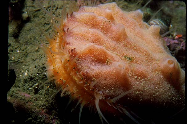
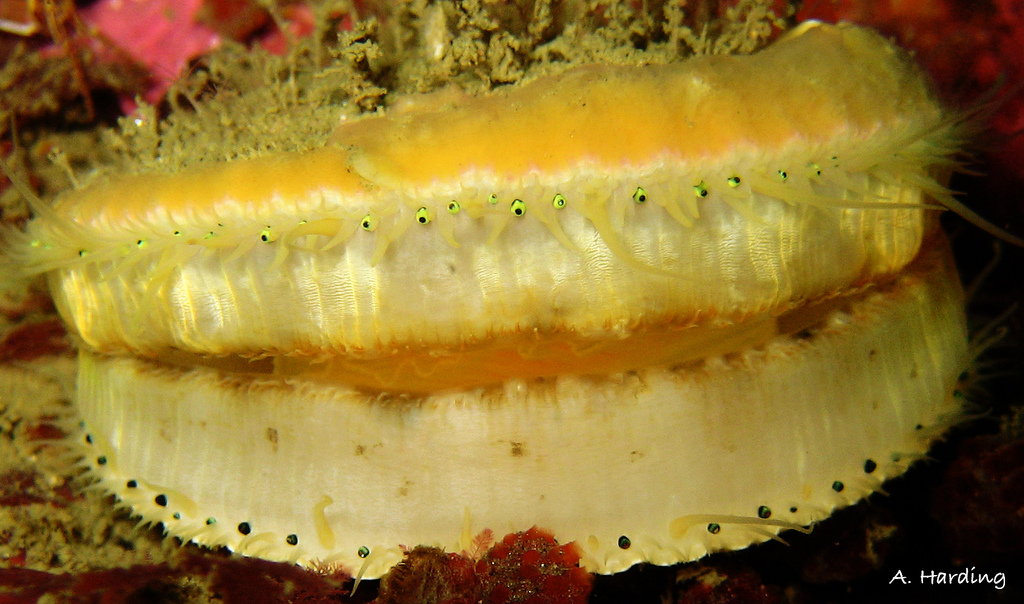
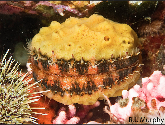
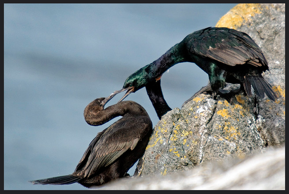
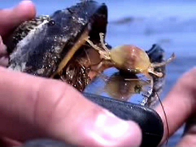
Jeremias, Carmen and Felix remove a pea crab from the mantle of a California Mussel.
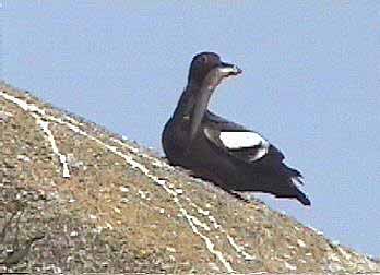
At Race Rocks there are many large mussels; (up to 30 cm) with such parasite inside.

&nbsp;

Domain Eukarya
Kingdom Animalia
Phylum Arthropoda
Class Crustacea
Order Decapoda
Family Pinnotheridae
Genus Fabia
Species subquadrata
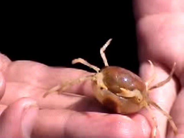
Common Name:Pea crab

Brief Definition

Pea/Mussel crabs are tiny creatures that live as symbionts, on or in the bodies of other invertebrates (bivalves)

Size

As their common name implies, Pea crabs are small creatures. The female pea crabs are distinctively larger than the male crabs, reachimg a size of 22mm (0.8in). The males however reach a size of 7.3mm (0.3in).

Habitat

Pea crabs occupy 2 different niches during their lifetime. Prior to and after their mating season, the adult female lives in a host. Host species include:

California mussels ( Mytilus californianus )

horse mussels ( Modiolus modiolus ).

Mytilus edulis

As well as other species of bivalves including scallops, oysters, cockles and clams.

The juvenile crabs also occupy a host before they become mature.

Range

These crabs live in mainly the northern hemisphere waters.

Including eastern and western U.S.(Akutan Pass, in the waters of Alaska to Ensenada.), Europe, Argentina and British Columbia, Canada.

It is found in 1 to 3% of California mussels along the central California coast, and 18% of mussels along Vancouver Island, BC, Canada.

Adaptation

Mussel crabs live in specific hosts because each crab responds positively to only certain chemicals that their hosts emit. In this way, they are able to infest the hosts that have the right conditions for them to survive. While in the host, these crabs do not posses an exokeleton. This is beacause the hosts provide them with protection against predators and other harmful external factors. However, when they leave their host to mate in the planktonic environment, the adult crabs grow an exoskeleton to protect their membranous carapace. These crabs also posses 10 legs, of which 2 of them develop into large and powerful claws to help fend off predators when exposed in the plankton, and to also help in the grasping of food.

Relationship with Host

The relationship that exists between the mussel crab and the bivalve is a symbiotic one. The advantage of this relationship is that the crab is protected while it scavenges the necessary nutrients needed by it, in the host. The crab however at times robs its host of a large mount of food and it also feeds off the protective mucus layers that cover the host’s tender tissues.This results in the mussel’s gills been injured. When this occurs the relationship becomes a parasitic one as the crab benefits while the host is affected negatively. Hence they are classified as parasites.

Precautions are taken when animals such as Mya arenaria, Placopecten magellanicus, Argopecten irradians and oysters are sold as to not have a pea crab inside it.

Reproduction and Lifecycle

The pea crabs’ life cycle has two distinct stages. These two stages are so different that in fact they were classified into two different genera.

The first stage comprises of the large, adult females that have soft membranous crapaces. These adults occupy a host each and they produce larvae that mature into the second stage. In the second stage, the offspring (larvae) of the female (that she had produced inside her host) grow up into adults of both sexes.Having reached maturity, they leave their hosts and join swarms in the water to mate. At this stage the pea crabs look more ‘traditional’. They have hard shells, strong legs (for swimming) and at the front of the carapace they have thick hair. Upon completion of mating, the female returns to her host. For a period of 21-25 weeks, she goes through 5 molts before reaching maturity. The female can inhabit here for up to a year, producing larvae from eggs that where fertilised by sperm from her single mating and then the cycle begins again. The mating takes place in late May.

Note: the male after mating dies.

References

Source 1: Pacific Coast Crabs and Shrimps by Gregory.C. Jensen, Ph.D

Source 2: Port Townsend Marine Science Center. Marine & Natural History Exihibits

Source 3: http://www.ptmsc.org/html/peacrabs.html

Source 4: http://life.bio.sunysb.edu/~jmatth/Science.htm

Source 5: http://www.pac.dfo-mpo.gc.ca/sci/shelldis/pages/pcbmu_e.htm

Source 6: http://www.indian-ocean.org/bioinformatics/crabs/crabs/tex1.html

Other Members of the Phylum Arthropoda at Race Rocks 
taxonomyiconReturn to the Race Rocks Taxonomy
and Image File
pearsonlogo2_f2The Race Rocks taxonomy is a collaborative venture originally started with the Biology and Environmental Systems students of Lester Pearson College UWC. It now also has contributions added by Faculty, Staff, Volunteers and Observers on the remote control webcams.

October 2003-  Michelle(PC)