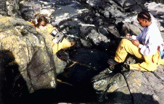
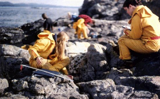
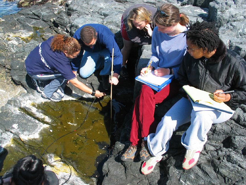
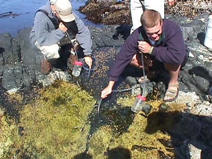
| BACKGROUND :It is intended that,students can access this file as a resource for an assignment in high school biology or college ecology coursers. For several years now, students of biology and environmental systems classes of Pearson College have been doing informal studies on the tidepools of Race Rocks. In April of 1996 we started to make some systematic records of some of the pools and establish a data base to which we could add in the future. The following represents the beginning of our tidepool work. |
| PURPOSE:by Michal Kozak
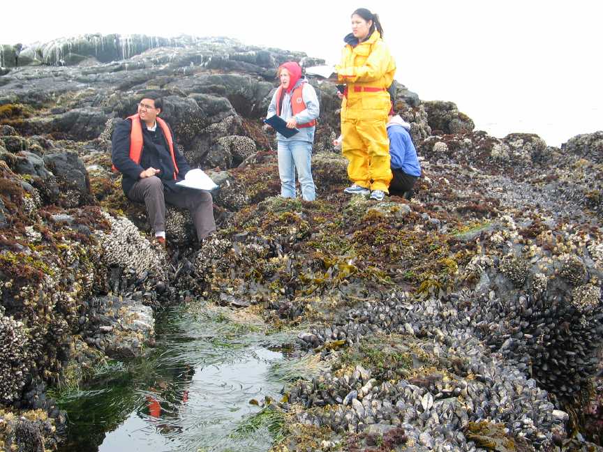
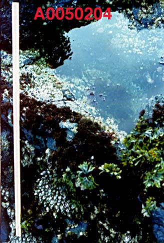
Tide pools are completely separate systems from that of the rocky shore. They form a sort of intermediate situation between the coastal sea and the well-drained intertidal zone, and thus give insights into factors controlling the structure and function of these two bordering systems. Tide pools are suitable for various student projects, similar to the one that we did. It is because of the amazing diversity of life and the wealth of physical, biological, and chemical processes in them. For instance, they show the importance of the desiccation factor on the open shore and they are also ideal observing pH and buffering phenomena. Their generally manageable proportion and simple ecosystems mean that thorough projects in tide pools can be undertaken in a short period. PROCEDURE: On Friday, 12th of April/96 during our block of environmental systems we went by boat to Race Rocks. We moored at the docks and then we went through across the island to the rocky shore. Besides numerous seagulls we saw there several tidepools. The tide level at that time was quite high (1.8 m), so at a lower tide we could have seen more tide pools. There we observed 3 different tide pools that were found close to the red peg, number 6. At each tidepool we measured the following :
We recorded our results and processed them ,thus trying to find general trends in the physical factors observed. The next Wednesday, we went to Race Rocks again. However, this time the tide was lower (0.9 m) which enabled us to observe tide pools at lower levels. We again followed the same procedure as described above. 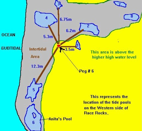
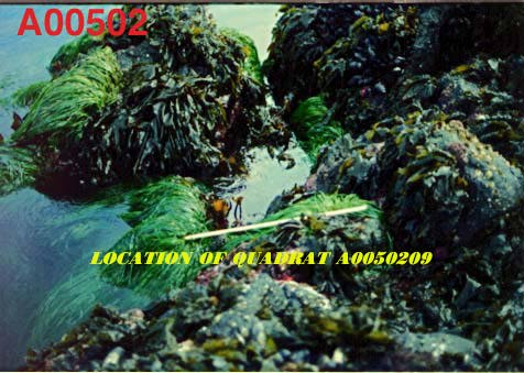
This map presents the horizontal distribution of the tide pools around a permanently installed reference peg on the Western side of Great Race Rock. We have over 15 of these reference pegs around the island. Many are used for subtidal transect work and surveys. Peg #6 is particularly well suited for intertidal work on this Western side of the island. Intertidal transect photos from the peg#5 location may be found at the Race Rocks Section of The Transect File. The magnetic compass bearings of the pools from the reference peg are listed below: Pool 3= 0 degrees. (compass bearing)
Pool 6= 205 degrees (compass bearing). . See the reference below to research work done on this pool by Dr. Anita Brinckmann Voss.
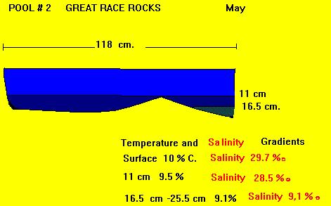
THE TEMPERATURE OF THE TIDE POOLS. Temperature of tide pools was measured for overall differences between pools and for stratification within pools BIOTIC FACTORS OF THE POOLS A species list was made of the pools and graphs were made to compare the numbers of plant and animal species in each pool.
A profile of the vertical distribution of the pools was done by Tamas in the spring of 1998. From this we can make hypothesis about correlations with vertical levels and differences in the pools. THE pH OF THE POOLS
PUBLICATIONS ON TIDEPOOLS:Brinckmann-Voss, A. 1996. Seasonality of Hydroids (Hydrozoa, Cnidaria) from an intertidal pool and adjacent subtidal habitats at Race Rocks, off Vancouver Island, Canada. Scientia Marina, 60 (1): 109-117This work done recently by Dr. Anita Brinckmann-Voss was in a tidepool (#6) adjacent to the ones we have been studying at Race Rocks. The purpose of her paper was “to provide information on the hydroids of a cold temperate tide pool with regard to seasonal occurrence, growth and regression, and reproductive periodicities.” She has reported an assemblage of 27 hydroid species and tracked their seasonal occurrence, growth, sexual maturity and systematics. Possible causes of hydroid species diversity are considered, including location of tide pool in an area of rapid tidal rapids, and shading by surfgrass and rock cliffs during low tide.Thomas, M.L.H.-1983. Marine and Coastal Systems of the Quoddy region, New Brunswick, Canada. Can. Spec.Publ.Fish.Aqua.Sci. 64: 1-306 This reference has been of use to us because it provides a classification scheme for tide pools and a series of charts and graphs which have provided useful models for our studies. Thomas notes that “Although there is a wealth of information on seashores, there is a paucity of information on tidal pools, particularly their functional aspects. There are no texts on pools and those on shores in general (Amos 1966; Carefoot 1977; Clayton 1974 ; Lewis 1964; Southward 1966; Stephenson and Stephenson 1972; Yonge 1949) provide little critical information about tidal pools. This undoubtedly results from the scarcity of scientific papers on tidal pools.”This file was prepared by the students of the Environmental Systems Classes and their teacher G.Fletcher. |
Category Archives: Ecological Monitoring
Transects for Environmental Monitoring at Race Rocks
CONTENTS: This section on Transects is composed of Several Parts:
1. This Page with background and some ideas.
2. Why do Transects.. overview and Techniques.
3. For a more in depth exercise on the Ecological Niche of organisms see this file: Ecological niche, The Empirical Model
4.See the following completed photographic transects:
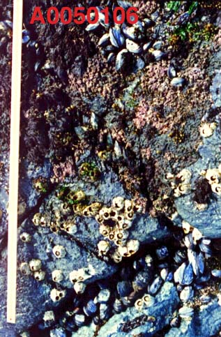
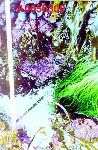
See Transect A0050101
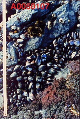
See Transect A0050102
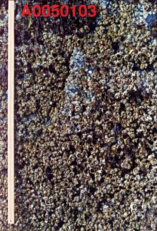
See Transect A0050103
BACKGROUND
The students and faculty of Lester B. Pearson College which is a member of the United World Colleges have used the ecological reserve and now the MPA of Race Rocks for studies of marine ecosystems, both sub-tidally and inter-tidally since1978. During that time a number of exercises have been developed to use in teaching ecological concepts in the International Baccalaureate Environmental Systems and Biology classes.
Transect Peg Locations on Race Rocks
Carmen’s Lab on Transects – kite Diagrams
1998 Class Photos and – Transects of Peg #`15
1999- Royal Roads Environmental management students visit Race Rocks
Underwater Transect at Race Rocks -Video
While using basic research techniques it has been possible to start to build up a library of information that can be more useful for determination of the effects of long term climatic changes or changes induced by humans, (anthropogenic). In addition this record may provide ideas to encourage others to apply the techniques to other ecosystems.
This program was developed at the 1995 BioQUEST Summer Workshop on Collaborative Learning, Peer Review, and Persuasion in Biology Education at Beloit College, WI. USA
See the following completed photographic transects:
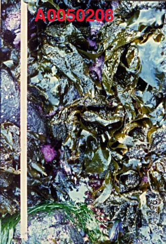
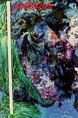
See Transect A0050101
See Transect A0050102
See Transect A0050103
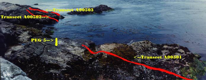
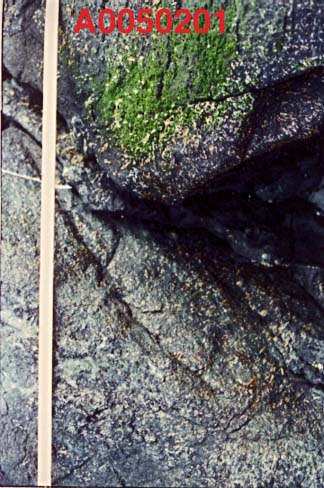
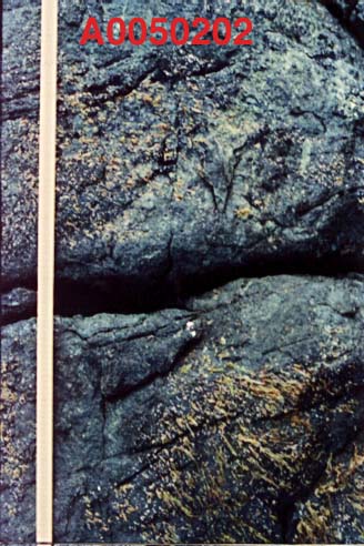
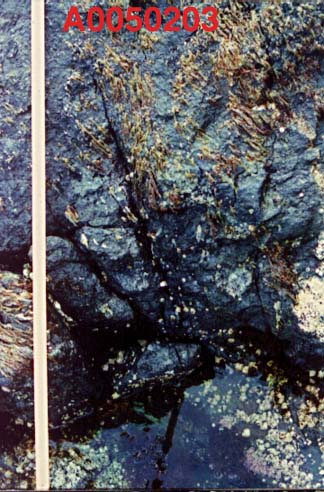
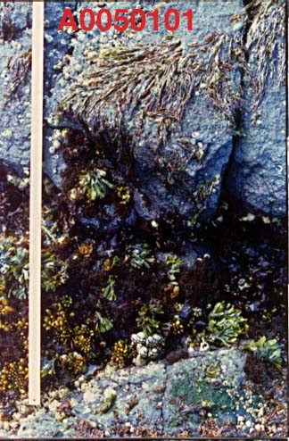
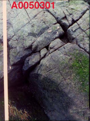
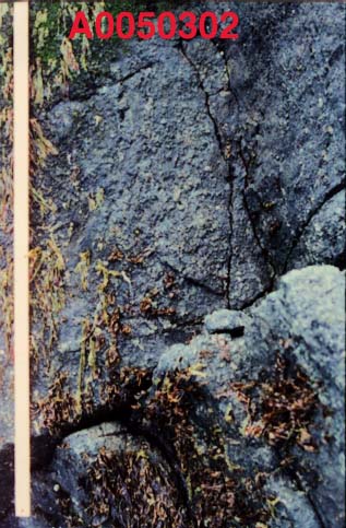
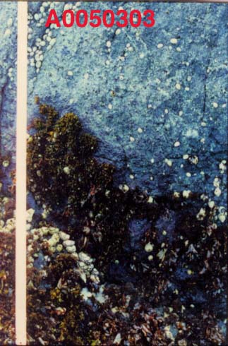
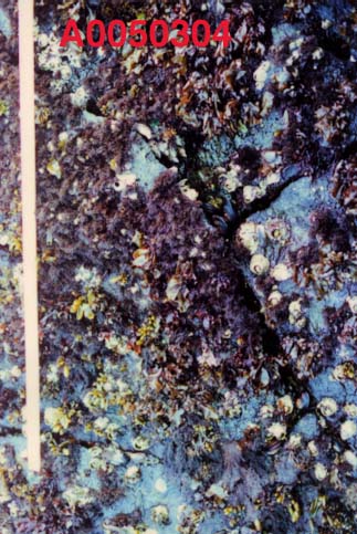
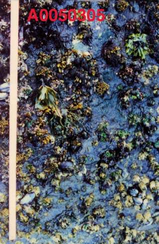
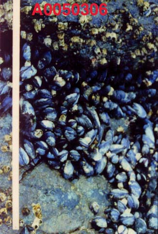
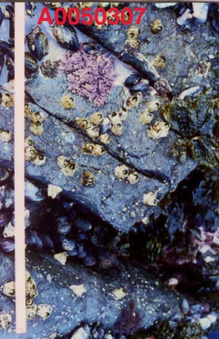
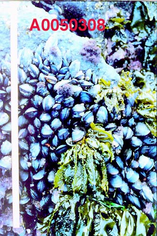
NUMBERING SYSTEM
A numbering system had to be developed that reflected the concept that this was only one of many that could be referenced from this site if individuals from around the world were willing to collaborate with us in building the project.
LOCATION….PEG NUMBER…TRANSECT NUMBER….QUADRAT NUMBER..
A0……..05…………01…………01………
Where:
| A0 | refers to the first site to be added to this WWW site |
| 05 | refers to the peg location ( we have 15 such locations permanently identified at the Race Rocks Ecological Reserve.) |
| 01 | refers to the first transect entered from this location. |
| 01 | refers to the first quadrat picture that you can access on this photographic strip. |
TIDAL LEVELS
Since the location of organisms in the intertidal zone is partially determined by tidal levels, that is one of the essential measurements given with our transect images. It is important to understand that the levels given here are based on the Canadian tide tables
Victoria Tide TablesThese are not calculated the same way as tables from the United States. To convert the elevations given here to conform to the US pattern in which 0.0 equals mean lower low water, subtract 0.8 meters from these Canadian readings.You may find further explanation on the operation of Tides in any marine biology or Oceanography text. One that may be useful is:
Seashore Life of the Northern Pacific Coast– by Eugene Kozloff, page 7-9.
For TIDAL Heights of Other LOCATIONS, use this link
SOME IDEAS FOR USE OF THESE TRANSECT PHOTOS
- Quantify the distribution of organisms
- Relate the distribution to the intertidal elevation
- Find out how to capture these images
- Use other technology to analyze the photos
- Study the mussels in greater depth
- Study other organisms from the transects in greater depth.
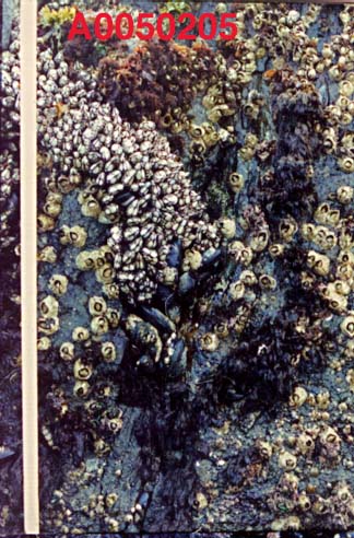
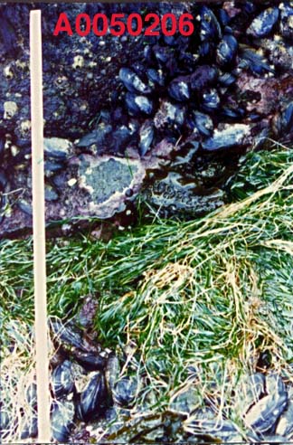
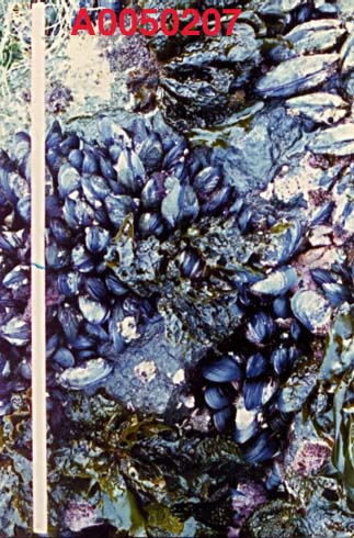
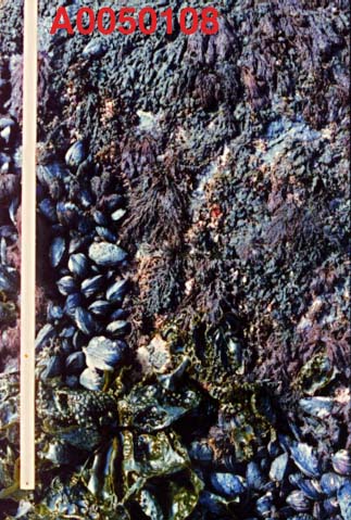
- Students in environmental systems will use this as a source to prepare for investigations in the intertidal zone when we have the opportunity to do a field lab at the ecological reserve. The photo strips also could be used by those living far from an ocean shore to study the relationship between abiotic or physical factors and organism distribution. Also by noting the location of certain species, for instance the mussels, M. californianus and then seeing where they would fit on a tidal level chart for the area (using the Victoria Tide Tables), students could calculate the length of times for submergence and emergence of the species in a week, a month, or a year. In addition they could compare the conditions in the winter months, with the extreme low tides occurring in the night with the conditions in the summer months when the low tides occur every two weeks in the daytime. Students should be encouraged to discuss the results of their investigations and pose further questions about conditions in the intertidal zone.
See Transect A0050101
See Transect A0050102
See Transect A0050103
THIS IS JUST A START!
By looking here you might get a few ideas of how you can do some interesting investigations using these pictures. But don’t stop there, we would like you to collaborate with us by adding ideas and new transects to our list. It would be excellent if someone living on another ocean shore with different intertidal zonation patterns could supply a similar set of photographs for comparison.Go back to techniques for directions on how to contribute
Transects on the west side of Race Rocks-2
LOCATION….PEG NUMBER…TRANSECT NUMBER….QUADRAT NUMBER..
A0………..05………….01……………01………
Where:
| A0 | refers to the first site to be added to this website |
| 05 | refers to the peg location ( we have 15 such locations permanently identified at the Race Rocks Ecological Reserve.) |
| 03 | refers to the third transect entered from this location. |
| 01 | refers to the first quadrat picture that you can access on this photographic strip. |
- Elevation 3.1 metres
- Elevation 2.9 metres
- Elevation 2.3metres
- Elevation 1.8 metres
- Elevation1.0 metres
- Elevation 0.6 metres
- Elevation 0.3 metres
- Elevation0.0 metres
- Elevation 0.0 metres
See Transect A0050101
See Transect A0050102
See Transect A0050103
_____________________________________________________________
Return to the Contents page for Environmental modelling with Transects..
Transects on the west side of Race Rocks-1
LOCATION….PEG NUMBER…TRANSECT NUMBER….QUADRAT NUMBER..
A0………..05………….01……………01………
Where:
| A0 | refers to the first site to be added to this website |
| 05 | refers to the peg location ( we have 15 such locations permanently identified at the Race Rocks Ecological Reserve.) |
| 03 | refers to the third transect entered from this location. |
| 01 | refers to the first quadrat picture that you can access on this photographic strip. |
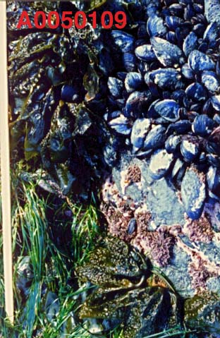
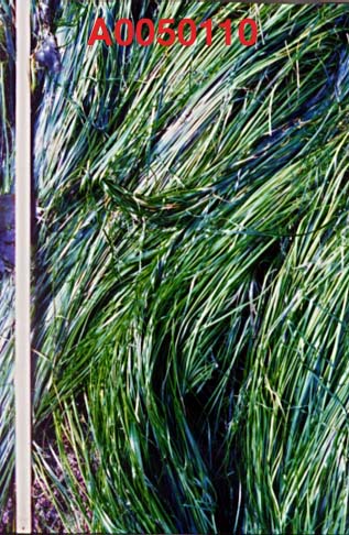
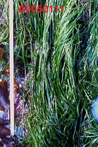
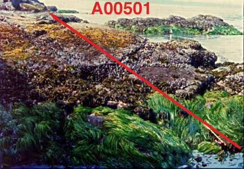 Transect A0050101
Elevation 3.7 metres
- Elevation 2.6 metres
- Elevation 2.3 metres
- Elevation 2.2 metres
- Elevation 1.9 metres
- Elevation 1.5 metres
- Elevation 1.2 metres
- Elevation 0.9 metres
- Elevation 1.1 metres
- Elevation 0.4 metres
- Elevation 1.1 metres
- Elevation0.0 metres
See Transect A0050101
See Transect A0050102
See Transect A0050103
Transects on the west side of Race Rocks-3
LOCATION….PEG NUMBER…TRANSECT NUMBER….QUADRAT NUMBER..
A0………..05………….01……………01………
Where:
| A0 | refers to the first site to be added to this website |
| 05 | refers to the peg location ( we have 15 such locations permanently identified at the Race Rocks Ecological Reserve.) |
| 03 | refers to the third transect entered from this location. |
| 01 | refers to the first quadrat picture that you can access on this photographic strip. |
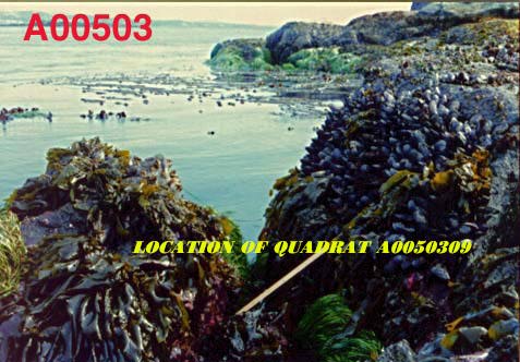
Transect A00503
Elevation 3.7 metres
- 2.3 metres
- 1.4 metres
- 0.0 metres
See Transect A0050101
See Transect A0050102
See Transect A0050103
Kalle Kallstrom’s extended essay on the Tidal Current meter
Race Rocks Sampling Programme
Long-term sampling programmes are often used to follow changes in the abundance of plants and animals over time. We will be looking at changes in the abundance of algae and invertebrates at Race Rocks. These changes will be examined with respect to changes in water temperature. The sampling method we will be using is called a stratified-random sample.
What is stratified random sampling?
In a stratified random sample we will sample the sea floor in a random manner, that is there will be no predetermined pattern to the sampling programme. The samples will be stratified because we will make sure that three depths are represented equally in our random samples.
What will we need?
Each dive pair will need
– a slate (with pencil)
– a pair of vernier calipers
– pre-mixed epoxy, and petersen discs
– a set of 20 random number
How will we sample?
We have established 6 permanent transects around Race Rocks. Each transect is 30 metres long and runs from the shallow subtidal to about 10m depth. Once a dive pair has located the transect they will be working on, a tape measure will be tied to the shallowest pin (the 0 metre pin) and laid out down to the last pin (30 metre pin).
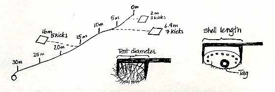
Before the dive, each dive pair will determine a set of 20 random numbers from a random number table (attached to these pages). There will be two numbers, both between 0 and 9. The first number will refer to the distance along the tape measure, let us say 6.9 metres (it will be the first two numbers, where-ever you start on the table, ie:69). The second number, let us say 7, will refer to the number of flipper kicks right or left of the line. The dive pair will swim along the tape locate the 6.9 mark, then left 7 kicks to the right or left of the 6.9 metre mark. After 7 kicks the diver drops the quadrat and starts to count all the invertebrates and seaweed in the quadrat.
While one diver does the counting and recording, the second diver will measure all of the sea urchins in the quadrat, recording the test diameter of each sea urchin to the nearest cm. Likewise the length of any abalone in the quadrat should also be measured, the abalone should also be tagged, using epoxy and a Petersen disc tag. The tag number should be recorded along with the length of the ablaone. Any abalone you see outside of the quadrat can also be measured and tagged.
Once the quadrat count and the measuring is completed, the dive pair returns to the tape measure, and repeats the process, using the next set of random numbers. In total divers will sample 20 quadrats between 0-10m (10 quadrats on the right side of the line, 10 quadrats on the left side), 20 quadrats between 10-20m and 20 quadrats between the 20-30m, for a total of 60 quadrats per transect. The transects will be sampled twice a year.
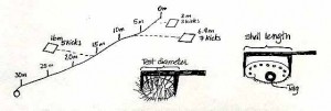 Once the dive pair has sampled 20 quadrats from between the 0-10 pins, they move down to the 10-20 metre pins and repeat the process, as time and air supply allow. If it is easier, three dive pairs can work on each transect line, one dive pair working in the 0-10m area, the next pair in the 10-20m area and the third pair in the 20-30m area. Dividing the transect into three areas is the stratified part of the sampling design, using the random number table is the random part of the sampling design.
Back at the College
Wash all the sampling gear you used with fresh water, and return to its appropriate place. Back in the lab you will need to wash the salt off your data sheet, and copy the sea urchin measurements and abalone tag/measurements onto the back of the data sheet for the section of the transect line you and your partner sampled. You will also need to make sure that all of your numbers are readable, and that you have filled in all of the blanks on the data sheet.
During later lab periods you will be entering this data, and calculating the average (mean) density of the animals and seaweed you counted along each transect line. Subsequent years of Pearson College students will continue this sampling programme to generate a long-term view of how invertebrate and algae abundance changes over time.
Temperature records.
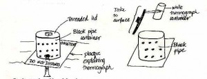 The Hobo thermograph that you will be installing, will automatically record water temperature. The temperatures are stored in the thermograph, and are down-loaded onto a programme that will be installed on the computers in the biology lab. The programme is very easy to use.
The thermograph will be installed in a black plastic pipe, bolted to the sea floor. The thermograph will be in a white water-tight container inside the pipe. To retrieve the thermograph divers will swim to the black pipe and using a filter wrench and a pipe wrench they will unscrew the lid on the black plastic pipe. Attached to the lid of the black plastic pipe, will be the white thermograph container. The divers bring the lid and the white thermograph container to the surface. DO NOT UNSCREW THE WHITE THERMOGRAPH CONTAINER UNDERWATER, THE COMPUTER INSIDE IT IS NOT WATER PROOF. THE THERMOGRAPH CAN ONLY BE REMOVED IN THE DRYNESS OF THE LAB.
Once the data have been down-loaded, the thermograph can be placed back in the white container, (the o-ring should be re-greased), the white container should be reattached the black lid, and on then the black re-screwed into the black pipe on the next dive. You will need to reset the thermograph right before you go diving.
Diagram of Hobo temperature apparatus appears here
Insert Random number table and data sheet.
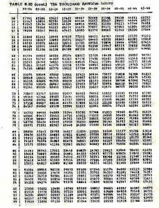
Following is a page of random numbers, you should make sure that you are comfortable using this table. Likewise there is a data sheet, please make sure that you are familiar with the species listed on the data sheet, and that you will be able to identify them underwater.
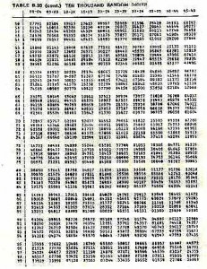 Random number table — 10,000 random numbers
27791 82504 33523
33147 46058 92388
67243 10545 40269
78176 70368 95523
70199 70547 94331
The first ten numbers in the last line are interpreted as: 7.0 m 1 kick, 9.9 m 7 kicks, 0.5 m 4 kicks, 7.9 m 4 kicks
TABLE B.39 (cont.) TEN THOUSAND RANDOM DIGITS
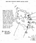
 Sample of one of the underwater recording projects. The numbers on the island represent pegs that are permanently imbedded in the rock. Transect lines go out from the pegs on designated bearings and belt transects are located at intervals indicated in meters. The records for these surveys are kept at Pearson College.
T = 1994-1995 permanent transects
 There will be other species of algae that we add to our list.
Sampling
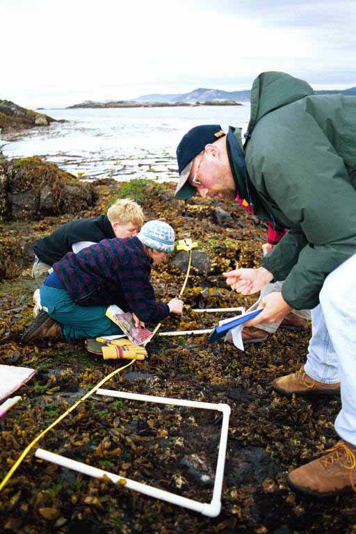
To sample the invertebrates at each of the permanently marked sites we will be using quadrats. Most of you will have done quadrat sampling before.
We will be using a random – sampling method, in which quadrats are placed randomly along / or near the transect line, and the selected invertebrates and algae in each quadrat will be counted. From these data we will calculate the mean (average) abundance as well as the variation in abundance that occurs at each site. These data will plotted in graphs which compare the abundance of each species over time, and with respect to changes in temperature.
We will go over the sampling methods prior to starting the project. Data will be recorded on data sheets pre-printed on underwater paper. An example of the type of data sheet we will be using is attached.
Race Rocks Long-Term Monitoring Programme
Dr. Jane Watson produced this report in the early 1980s.
What is the purpose of long-term monitoring projects?
Long-term monitoring projects are often used to follow changes in community composition or structure that occur over time. In this case you will be looking at natural changes in marine algae and invertebrate populations with respect to both long and short-term changes in water temperature.
How will this project be carried out?
You will be helping to establish the study sites which ultimately Pearson college will monitor two to three times a year. At least four of these sites will be at Race Rocks, others will be established at other sites that Pearson College divers visit regularly.
What will this involve?
Over the next three months we will be putting the permanently marked transects in. Once we have established all of the transects we will start to sample them. On each permanently marked transect Coast-watch divers will use randomly placed quadrats to estimate the abundance of selected invertebrates and algae.
In the lab the data will be entered and analyzed. These data should show how the abundance of many of many marine plants and animals change over time.
We will also be installing an underwater thermograph. This small instrument will record water temperature at predetermined intervals. Several times a year Pearson college divers will retrieve the instrument and down-load the data onto a computer. Changes in the composition of the marine community can then be examined with respect to mean temperatures, extreme temperatures and so on.
In addition to counting the abundance of marine invertebrates and algae, we will be tagging abalone, in an attempt to follow growth and mortality of individual abalone. We will also be measuring urchins which will allow us to follow changes in the population structure over time.
What will you need to know to sample these sites?
There are a number of plant and invertebrate species that you will need to be able to identify before we can sample the sites. You will also need to know how to sample using a quadrat, tag abalone and use vernier callipers… not exactly difficult stuff.
You will also need to know how to enter and analyze the data you collect. We will set things up so that this is straightforward. At the end of the school term you will be able to plot the mean abundance of the organisms we sample at all of our permanent transects. In subsequent years other Pearson College divers will continue to sample these sites.
Invertebrates
Phylum Echinodermata
Red urchin – Strongylocentrotus franciscanus
This is the most abundant of the urchins, it is unmistakable, being big and red. We will count the number of red urchins in each quadrat, as well as measuring the test diameter of the urchins. This will be done with vernier callipers. By measuring the size of the urchin tests we will be able to trace the settlement of new “recruits” and follow their growth.
Green urchin – S. droebachiensis
This is the smaller green urchin that is quite common in sheltered areas. We will count green urchins, but not measure them, unless they are very abundant at any of our sites.
Purple urchin – S. purpuratus
A small purple urchin that is generally found in the very shallow subtidal, and sometimes in the intertidal. If it occurs on any of our sites we will count them only.
Green urchins – S. droebachiensis
A small green urchin that is generally found in more sheltered waters, we will probably not encounter too many green urchins.
Giant sea cucumber – Parastichopus californicus
A large browny red sea cucumber, These are generally found in sheltered areas, or in water depths of greater than 10m. They are found on both hard and soft-bottoms.
Orange sea cucumber – Cucumaria miniata
This cucumber has a browny red body and bright orange tentacles. It is found in crevices wifli its tentacles extending beyond the crevice.
Sunflower star – Pycnopodia helianthoides
The largest of the sea stars, it can be up to lm in diameter, it comes in a variety of colours, usually orangy brown. It has up to 24 legs.
Leather star – Dermasterias imbricata
The leather star has a red back with greeny makings. It derives its name from its ieather-like texture. If you smell it (no not underwater) it has a gunpowder/garlic smell.
Beach star – Pisaster ochraceus
Yellow or purple, generally intertidal, but also found subtidally at some locations .
Painted star – Orthasterias khoeleri
Orange pink and purple, a very attractive sea star that occurs subtidally on rocky bottoms.
Blood star – Henticia spp.
This bright red, star is very common on both rocky and soft-bottomed areas.
Basket star – Gorganocephalus eucnemis
This species usually occurs in deep water, but Race Rocks is unique in having this species in shallow subtidal water.
Phylum Mollusca
Abalone – Haliotois kamtschatkana
The pinto abalone occurs from the lower intertidal to depths of about 10m. We will count, measure and tag all of the abalone we encounter. When tagged abalone are re-encountered they will be re-measured to follow growth in abalone.
Red turban snail – Astraea gibbersoa
A medium-sized snail that is very common on coralline algae. It has a hard operculum, and a shell that becomes covered with coralline algae.
Gumboot chiton – Cryptochiton stelleri
‘Ite largest chiton on our coast. You cannot see the 8 shell or plates that make up the gumboot chiton’s shell, they are hidden beneath the pinky brown tissue on the dorsal surface.
Cnidaria
Plumose anenome – Metridum senile
A very abundant bright white anenome, that does particularly well in high current areas. We will count anemones as we encounter them.
There will be other invertebrates added to this list once we determine which species are representative of the areas we are sampling.
Brown Algae
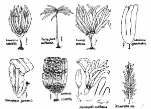
Kelps – Laminariales
 Bull kelp – Nereocystis luetkeana
Bull kelp is an annual species, it grows rapidly in areas that are highly disturbed. Bull kelp forms a floating canopy, it is very common at Race Rocks.
Tree kelp – Ptrerygophora californica
Tree kelp looks very much like a tree. It is a perennial species that lives in excess of 17 years. Pterygophora can be aged by cutting it down and counting the rings in its stalk or stipe. We will be tagging tree kelp on one of the transects at Race Rocks this will allow us to look at the persistence of tree kelp
Eisenia arborea
Eisenia looks very much Pterygophora, except that it has blades which are serrated at the edges, and the blades grow in two “bunches” at the top of the plant.
Laminafia setcheIlii
Laminaria groenlandica
These two species do not have a common name. Laminaria setchellii found in similar areas to Pterygophora, except that Laminaria setchellii is generally found in slightly more exposed areas.
Laminaria groenlandica is found in more sheltered areas. It looks quite different than Laminaria setchellii, since the two species are found in different areas you should have no trouble sorting them out.
Costaria costata
Costaria is really distinctive, it has three ribs on one side and two ribs on the other. It is generally an annual species but frequently manages to overwinter.
Acid weed – Desmarestia spp.
Acid weed is an annual species, which has a very “weedy” life history, it grows in highly disturbed areas, and is one of the first species to grow in areas that have been disturbed. It is very hard to count, because it forms a blanket over the sea floor, to count it you have to go down to the holdfast.
Pleurophycus gardneri
This species is generally found in very shallow areas in wave-washed areas. It is very distinctive.
There will be other species of algae that we add to our list.
SAMPLING
To sample the invertebrates at each of the permanently marked sites we will be using quadrats. Most of you will have done quadrat sampling before.
We will be using a random – sampling method, in which quadrats are placed randomly along / or near the transect line, and the selected invertebrates and algae in each quadrat will be counted. From these data we will calculate the mean (average) abundance as well as the variation in abundance that occurs at each site. These data will plotted in graphs which compare the abundance of each species over time, and with respect to changes in temperature.
We will go over the sampling methods prior to starting the project. All data will be recorded on data sheets pre-printed on underwater paper. An example of the type of data sheet we will be using is attached.
Race Rocks Long-Term Monitoring Program
What is the purpose of long-term monitoring projects?
Long-term monitoring projects are often used to follow changes in community composition or structure that occur over time. In this case you will be looking at natural changes in marine algae and invertebrate populations with respect to both long and short-term changes in water temperature.
How will this project be carried out?
You will be helping to establish the study sites which ultimately Pearson college will monitor two to three times a year. At least four of these sites will be at Race Rocks, others will be established at other sites that Pearson College divers visit regularly.
What will this involve?
Over the next three months we will be putting the permanently marked transects in. Once we have established all of the transects we will start to sample them. On each permanently marked transect Coast-watch divers will use randomly placed quadrats to estimate the abundance of selected invertebrates and algae.
In the lab the data will be entered and analyzed. These data should show how the abundance of many of many marine plants and animals change over time.
We will also be installing an underwater thermograph. This small instrument will record water temperature at predetermined intervals. Several times a year Pearson college divers will retrieve the instrument and down-load the data onto a computer. Changes in the composition of the marine community can then be examined with respect to mean temperatures, extreme temperatures and so on.
In addition to counting the abundance of marine invertebrates and algae, we will be tagging abalone, in an attempt to follow growth and mortality of individual abalone. We will also be measuring urchins which will allow us to follow changes in the population structure over time.
What will you need to know to sample these sites?
There are a number of plant and invertebrate species that you will need to be able to identify before we can sample the sites. You will also need to know how to sample using a quadrat, tag abalone and use vernier callipers… not exactly difficult stuff.
You will also need to know how to enter and analyze the data you collect. We will set things up so that this is straightforward. At the end of the school term you will be able to plot the mean abundance of the organisms we sample at all of our permanent transects. In subsequent years other Pearson College divers will continue to sample these sites.
Some species you will need to know
Invertebrates
Phylum Echinodermata
Red urchin – Strongylocentrotus franciscanus
This is the most abundant of the urchins, it is unmistakable, being big and red. We will count the number of red urchins in each quadrat, as well as measuring the test diameter of the urchins. This will be done with vernier callipers. By measuring the size of the urchin tests we will be able to trace the settlement of new “recruits” and follow their growth.
Green urchin – S. droebachiensis
This is the smaller green urchin that is quite common in sheltered areas. We will count green urchins, but not measure them, unless they are very abundant at any of our sites.
Purple urchin – S. purpuratus
A small purple urchin that is generally found in the very shallow subtidal, and sometimes in the intertidal. If it occurs on any of our sites we will count them only.
Green urchins – S. droebachiensis
A small green urchin that is generally found in more sheltered waters, we will probably not encounter too many green urchins.
Giant sea cucumber – Parastichopus californicus
A large browny red sea cucumber, These are generally found in sheltered areas, or in water depths of greater than 10m. They are found on both hard and soft-bottoms.
Orange sea cucumber – Cucumaria miniata
This cucumber has a browny red body and bright orange tentacles. It is found in crevices wifli its tentacles extending beyond the crevice.
Sunflower star – Pycnopodia helianthoides
The largest of the sea stars, it can be up to lm in diameter, it comes in a variety of colours, usually orangy brown. It has up to 24 legs.
Leather star – Dermasterias imbricata
The leather star has a red back with greeny makings. It derives its name from its ieather-like texture. If you smell it (no not underwater) it has a gunpowder/garlic smell.
Beach star – Pisaster ochraceus
Yellow or purple, generally intertidal, but also found subtidally at some locations .
Painted star – Orthasterias khoeleri
Orange pink and purple, a very attractive sea star that occurs subtidally on rocky bottoms.
Blood star – Henticia spp.
This bright red, star is very common on both rocky and soft-bottomed areas.
Basket star – Gorganocephalus eucnemis
This species usually occurs in deep water, but Race Rocks is unique in having this species in shallow subtidal water.
Phylum Mollusca
Abalone – Haliotois kamtschatkana
The pinto abalone occurs from the lower intertidal to depths of about 10m. We will count, measure and tag all of the abalone we encounter. When tagged abalone are re-encountered they will be re-measured to follow growth in abalone.
Red turban snail – Astraea gibbersoa
A medium-sized snail that is very common on coralline algae. It has a hard operculum, and a shell that becomes covered with coralline algae.
Gumboot chiton – Cryptochiton stelleri
‘Ite largest chiton on our coast. You cannot see the 8 shell or plates that make up the gumboot chiton’s shell, they are hidden beneath the pinky brown tissue on the dorsal surface.
Cnidaria
Plumose anenome – Metridum senile
A very abundant bright white anenome, that does particularly well in high current areas. We will count anemones as we encounter them.
There will be other invertebrates added to this list once we determine which species are representative of the areas we are sampling.
Brown Algae
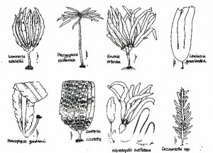 Kelps – Laminariales
Bull kelp – Nereocystis luetkeana
Bull kelp is an annual species, it grows rapidly in areas that are highly disturbed. Bull kelp forms a floating canopy, it is very common at Race Rocks.
Tree kelp – Ptrerygophora californica
Tree kelp looks very much like a tree. It is a perennial species that lives in excess of 17 years. Pterygophora can be aged by cutting it down and counting the rings in its stalk or stipe. We will be tagging tree kelp on one of the transects at Race Rocks this will allow us to look at the persistence of tree kelp
Eisenia arborea
Eisenia looks very much Pterygophora, except that it has blades which are serrated at the edges, and the blades grow in two “bunches” at the top of the plant.
Laminafia setcheIlii
Laminaria groenlandica
These two species do not have a common name. Laminaria setchellii found in similar areas to Pterygophora, except that Laminaria setchellii is generally found in slightly more exposed areas.
Laminaria groenlandica is found in more sheltered areas. It looks quite different than Laminaria setchellii, since the two species are found in different areas you should have no trouble sorting them out.
Costaria costata
Costaria is really distinctive, it has three ribs on one side and two ribs on the other. It is generally an annual species but frequently manages to overwinter.
Acid weed – Desmarestia spp.
Acid weed is an annual species, which has a very “weedy” life history, it grows in highly disturbed areas, and is one of the first species to grow in areas that have been disturbed. It is very hard to count, because it forms a blanket over the sea floor, to count it you have to go down to the holdfast.
Pleurophycus gardneri
This species is generally found in very shallow areas in wave-washed areas. It is very distinctive.
There will be other species of algae that we add to our list.
SAMPLING
To sample the invertebrates at each of the permanently marked sites we will be using quadrats. Most of you will have done quadrat sampling before.
We will be using a random – sampling method, in which quadrats are placed randomly along / or near the transect line, and the selected invertebrates and algae in each quadrat will be counted. From these data we will calculate the mean (average) abundance as well as the variation in abundance that occurs at each site. These data will plotted in graphs which compare the abundance of each species over time, and with respect to changes in temperature.
We will go over the sampling methods prior to starting the project. All data will be recorded on data sheets pre-printed on underwater paper. An example of the type of data sheet we will be using is attached.
Long-term sampling programmes are often used to follow changes in the abundance of plants and animals over time. We will be looking at changes in the abundance of algae and invertebrates at Race Rocks. These changes will be examined with respect to changes in water temperature. The sampling method we will be using is called a stratified-random sample.
What is stratified random sampling?
In a stratified random sample we will sample the sea floor in a random manner, that is there will be no predetermined pattern to the sampling programme. The samples will be stratified because we will make sure that three depths are represented equally in our random samples.
What will we need?
Each dive pair will need
– a 30m tape measure
– a 0.7m X 0.7m quadrat (0.5m squared)
– a clip board and data sheet (with pencil)
– a slate (with pencil)
– a pair of vernier calipers
– pre-mixed epoxy, and petersen discs
– a set of 20 random number
How will we sample?
We have established 6 permanent transects around Race Rocks. Each transect is 30 metres long and runs from the shallow subtidal to about 10m depth. Once a dive pair has located the transect they will be working on, a tape measure will be tied to the shallowest pin (the 0 metre pin) and laid out down to the last pin (30 metre pin).
Before the dive, each dive pair will determine a set of 20 random numbers from a random number table (attached to these pages). There will be two numbers, both between 0 and 9. The first number will refer to the distance along the tape measure, let us say 6.9 metres (it will be the first two numbers, where-ever you start on the table, ie:69). The second number, let us say 7, will refer to the number of flipper kicks right or left of the line. The dive pair will swim along the tape locate the 6.9 mark, then left 7 kicks to the right or left of the 6.9 metre mark. After 7 kicks the diver drops the quadrat and starts to count all the invertebrates and seaweed in the quadrat.
While one diver does the counting and recording, the second diver will measure all of the sea urchins in the quadrat, recording the test diameter of each sea urchin to the nearest cm. Likewise the length of any abalone in the quadrat should also be measured, the abalone should also be tagged, using epoxy and a Petersen disc tag. The tag number should be recorded along with the length of the ablaone. Any abalone you see outside of the quadrat can also be measured and tagged.
Once the quadrat count and the measuring is completed, the dive pair returns to the tape measure, and repeats the process, using the next set of random numbers. In total divers will sample 20 quadrats between 0-10m (10 quadrats on the right side of the line, 10 quadrats on the left side), 20 quadrats between 10-20m and 20 quadrats between the 20-30m, for a total of 60 quadrats per transect. The transects will be sampled twice a year.
Once the dive pair has sampled 20 quadrats from between the 0-10 pins, they move down to the 10-20 metre pins and repeat the process, as time and air supply allow. If it is easier, three dive pairs can work on each transect line, one dive pair working in the 0-10m area, the next pair in the 10-20m area and the third pair in the 20-30m area. Dividing the transect into three areas is the stratified part of the sampling design, using the random number table is the random part of the sampling design.
Back at the College
Wash all the sampling gear you used with fresh water, and return to its appropriate place. Back in the lab you will need to wash the salt off your data sheet, and copy the sea urchin measurements and abalone tag/measurements onto the back of the data sheet for the section of the transect line you and your partner sampled. You will also need to make sure that all of your numbers are readable, and that you have filled in all of the blanks on the data sheet.
During later lab periods you will be entering this data, and calculating the average (mean) density of the animals and seaweed you counted along each transect line. Subsequent years of Pearson College students will continue this sampling programme to generate a long-term view of how invertebrate and algae abundance changes over time.
Following is a page of random numbers, you should make sure that you are comfortable using this table. Likewise there is a data sheet, please make sure that you are familiar with the species listed on the data sheet, and that you will be able to identify them underwater.
Random number table — 10,000 random numbers
33147 46058 92388
67243 10545 40269
78176 70368 95523
70199 70547 94331
The first ten numbers in the last line are interpreted as: 7.0 m 1 kick, 9.9 m 7 kicks, 0.5 m 4 kicks, 7.9 m 4 kicks
TABLE B.39 (cont.) TEN THOUSAND RANDOM DIGITS
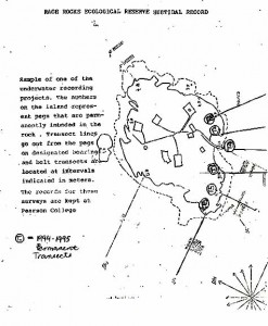 Sample of one of the underwater recording projects. The numbers on the island represent pegs that are permanently imbedded in the rock. Transect lines go out from the pegs on designated bearings and belt transects are located at intervals indicated in meters. The records for these surveys are kept at Pearson College.
T = 1994-1995 permanent transects
 There will be other species of algae that we add to our list.
Sampling
To sample the invertebrates at each of the permanently marked sites we will be using quadrats. Most of you will have done quadrat sampling before.
We will be using a random – sampling method, in which quadrats are placed randomly along / or near the transect line, and the selected invertebrates and algae in each quadrat will be counted. From these data we will calculate the mean (average) abundance as well as the variation in abundance that occurs at each site. These data will plotted in graphs which compare the abundance of each species over time, and with respect to changes in temperature.
We will go over the sampling methods prior to starting the project. Data will be recorded on data sheets pre-printed on underwater paper.
Long-term sampling programmes are often used to follow changes in the abundance of plants and animals over time. We will be looking at changes in the abundance of algae and invertebrates at Race Rocks. These changes will be examined with respect to changes in water temperature. The sampling method we will be using is called a stratified-random sample.
What is stratified random sampling?
In a stratified random sample we will sample the sea floor in a random manner, that is there will be no predetermined pattern to the sampling programme. The samples will be stratified because we will make sure that three depths are represented equally in our random samples.
What will we need?
Each dive pair will need
– a 30m tape measure
– a 0.7m X 0.7m quadrat (0.5m squared)
– a clip board and data sheet (with pencil)
– a slate (with pencil)
– a pair of vernier calipers
– pre-mixed epoxy, and petersen discs
– a set of 20 random number
We have established 6 permanent transects around Race Rocks. Each transect is 30 metres long and runs from the shallow subtidal to about 10m depth. Once a dive pair has located the transect they will be working on, a tape measure will be tied to the shallowest pin (the 0 metre pin) and laid out down to the last pin (30 metre pin).
Before the dive, each dive pair will determine a set of 20 random numbers from a random number table (attached to these pages). There will be two numbers, both between 0 and 9. The first number will refer to the distance along the tape measure, let us say 6.9 metres (it will be the first two numbers, where-ever you start on the table, ie:69). The second number, let us say 7, will refer to the number of flipper kicks right or left of the line. The dive pair will swim along the tape locate the 6.9 mark, then left 7 kicks to the right or left of the 6.9 metre mark. After 7 kicks the diver drops the quadrat and starts to count all the invertebrates and seaweed in the quadrat.
While one diver does the counting and recording, the second diver will measure all of the sea urchins in the quadrat, recording the test diameter of each sea urchin to the nearest cm. Likewise the length of any abalone in the quadrat should also be measured, the abalone should also be tagged, using epoxy and a Petersen disc tag. The tag number should be recorded along with the length of the ablaone. Any abalone you see outside of the quadrat can also be measured and tagged.
Once the quadrat count and the measuring is completed, the dive pair returns to the tape measure, and repeats the process, using the next set of random numbers. In total divers will sample 20 quadrats between 0-10m (10 quadrats on the right side of the line, 10 quadrats on the left side), 20 quadrats between 10-20m and 20 quadrats between the 20-30m, for a total of 60 quadrats per transect. The transects will be sampled twice a year.
Once the dive pair has sampled 20 quadrats from between the 0-10 pins, they move down to the 10-20 metre pins and repeat the process, as time and air supply allow. If it is easier, three dive pairs can work on each transect line, one dive pair working in the 0-10m area, the next pair in the 10-20m area and the third pair in the 20-30m area. Dividing the transect into three areas is the stratified part of the sampling design, using the random number table is the random part of the sampling design.
Back at the College
Wash all the sampling gear you used with fresh water, and return to its appropriate place. Back in the lab you will need to wash the salt off your data sheet, and copy the sea urchin measurements and abalone tag/measurements onto the back of the data sheet for the section of the transect line you and your partner sampled. You will also need to make sure that all of your numbers are readable, and that you have filled in all of the blanks on the data sheet.
During later lab periods you will be entering this data, and calculating the average (mean) density of the animals and seaweed you counted along each transect line. Subsequent years of Pearson College students will continue this sampling programme to generate a long-term view of how invertebrate and algae abundance changes over time.
Insert Random number table and data sheet.
Following is a page of random numbers, you should make sure that you are comfortable using this table. Likewise there is a data sheet, please make sure that you are familiar with the species listed on the data sheet, and that you will be able to identify them underwater.
Random number table — 10,000 random numbers
27791 82504 33523
33147 46058 92388
67243 10545 40269
78176 70368 95523
70199 70547 94331
The first ten numbers in the last line are interpreted as: 7.0 m 1 kick, 9.9 m 7 kicks, 0.5 m 4 kicks, 7.9 m 4 kicks
TABLE B.39 (cont.) TEN THOUSAND RANDOM DIGITS
T = 1994-1995 permanent transects
There will be other species of algae that we add to our list.
Sampling
To sample the invertebrates at each of the permanently marked sites we will be using quadrats. Most of you will have done quadrat sampling before.
We will be using a random – sampling method, in which quadrats are placed randomly along / or near the transect line, and the selected invertebrates and algae in each quadrat will be counted. From these data we will calculate the mean (average) abundance as well as the variation in abundance that occurs at each site. These data will plotted in graphs which compare the abundance of each species over time, and with respect to changes in temperature.
We will go over the sampling methods prior to starting the project. Data will be recorded on data sheets pre-printed on underwater paper. An example of the type of data sheet we will be using is attached.
Jane Watson
Faculty of Science &Technology
900 fifth Street, Nanaimo,
British Columbia, Canada V9R 5S5
Tel (250) 741-2300 – Fox (250) 755-8749 http:llwww.mala.bc.cal

