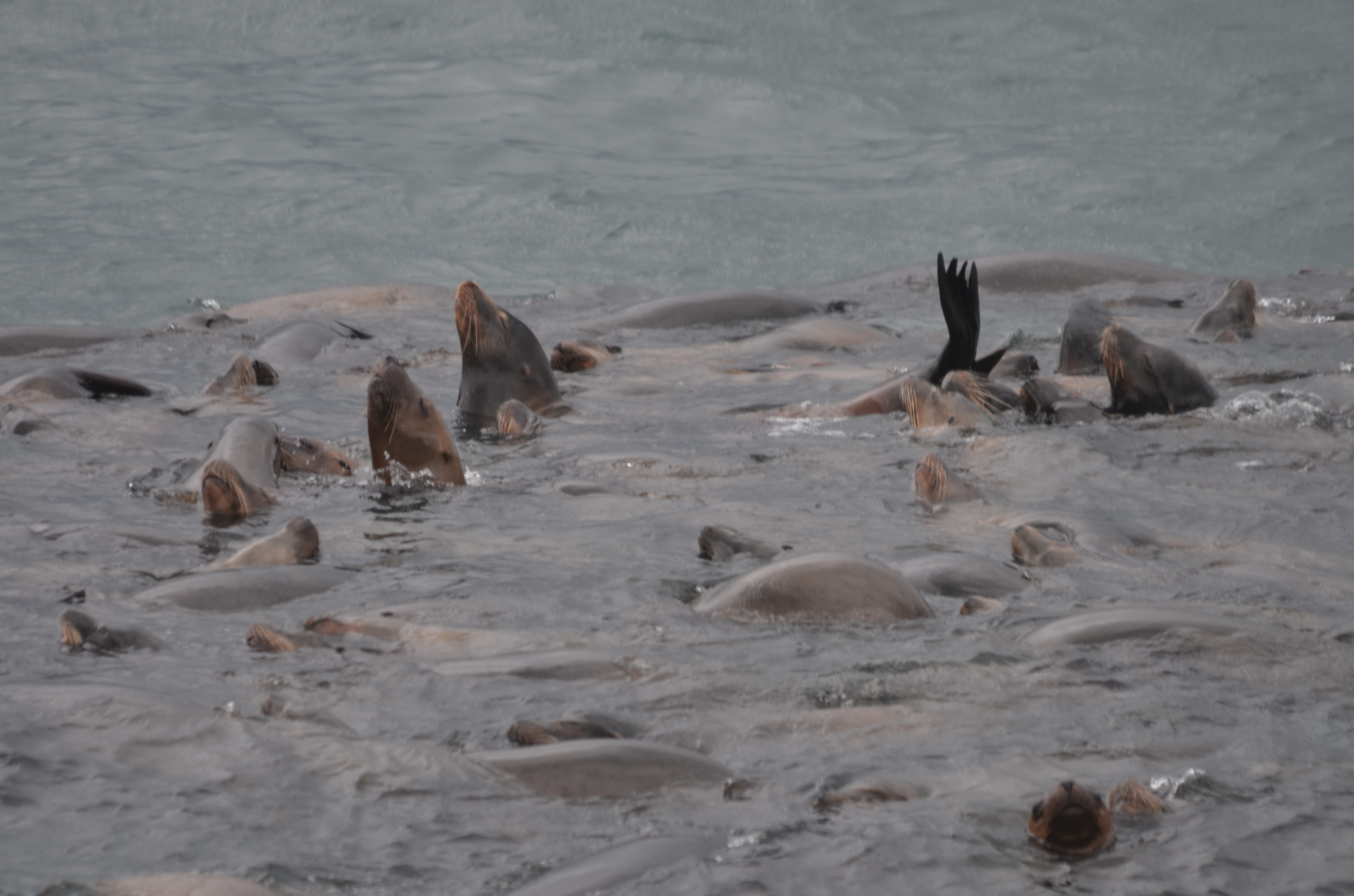
Ryan Murphy took this high resolution image, ideal for getting accurate census counts, on November 20. 2009. The population is pretty well all Thayer’s Gulls as far as I can determine. Since it is so large it will take several seconds to load. Click to enlarge.
Category Archives: Ecology
Calendula officinalis: marigold–The Race Rocks Taxonomy
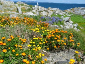
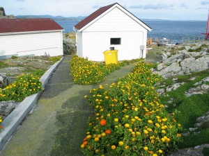
Although introduced to Race Rocks by lightkeepers to brighten up their garden years ago, Calendula sp.is an interesting exotic since because of the ocean moderated temperature of the Ecological Reserve, it blooms at Race Rocks every month of the year. The reason it is so successful there is probably that it is not grazed by gulls or geese.
Also see the notation and images by Ecoguardian Anne Stewart, Sept 13 2015.
Scientific classification
Kingdom: Plantae
(unranked): Eudicots
(unranked): Asterids
Order: Asterales
Family: Asteraceae
Subfamily: Asteroideae
Tribe: Calenduleae
Genus: Calendula
species: officinalis
Other Angiosperms (flowering plants) at Race Rock
and Image File |
 The Race Rocks taxonomy is a collaborative venture originally started with the Biology and Environmental Systems students of Lester Pearson College UWC. It now also has contributions added by Faculty, Staff, Volunteers and Observers on the remote control webcams. The Race Rocks taxonomy is a collaborative venture originally started with the Biology and Environmental Systems students of Lester Pearson College UWC. It now also has contributions added by Faculty, Staff, Volunteers and Observers on the remote control webcams. |
Ecological Niche -the Empirical Model
Return to the Contents page for Environmental modelling with Transects..
| BACKGROUND | HISTORICAL TREATMENT of the ECOLOGICAL NICHE | |
| Joseph Grinnell | 1917 | the habitats and habits of birds |
| Charles Elton | 1927 | the species’ place in the biological environment, its relationship to food and predators. |
| G.F. Gause | 1934 | the intensity of competition between species suggest the degree to which their niches overlapped |
| David Lack | 1947 | realized that niche relationships could provide a basis for evolutionary diversification of species |
| G.E.Hutchinson | 1959 | was the first to define the niche concept formally as the activity range of each species along every dimension of the environment. |
G. E. Hutchinson on the Niche Concept: In 1957, in a paper entitled “the Niche Concept by G. E. Hutchinson defined the niche concept formally. One could describe the activity range along every dimension of the environment. Physical and chemical factors such as temperature, humidity, salinity, and oxygen concentration, and biological factors such as prey species and resting background against which an individual may escape detection by predators, could be determined. Each of these dimensions could be thought of as one of n-dimensions in space. Visualizing a space with more than three dimensions is difficult, since the concept of the n-dimensional niche is an abstraction. We may, however, deal with multi-dimensional concepts mathematically and statistically, depicting their essence by physical or graphical representations in three or fewer dimensions.
Ricklefs (1996) notes that “… for example, a graph relating biological activity to a single environmental gradient represents the distribution of a species’ activity along one niche dimension. The level of activity, whether oxygen metabolism as a function of temperature or consumption rate as function of prey size, conveys the ability of an individual to exploit resources in a particular part of the niche space and, conversely, the degree to which the environment can support the population of that species. In two dimensions the individuals niche may be depicted as a hill, with contours representing the various levels of biological activity. In three dimensions, we must think of a cloud in space whose density conveys niche utilization. Beyond three the mind boggles.”
Please see Hutchinson, R.E. 1957. Concluding remarks. Cold Spring Harbor. Symp. Quant. Biol. 22: 415-427.
Paraphrased from Ecology by R. E. Ricklefs 1996.
Hutchinson was the first to formally quantify the niche concept in terms of geometric space. For example, suppose the distribution of a given species of tree squirrel is determined primarily by 3 variables: branch diameter, acorn size and temperature. The “level of activity” describes the ability of the individual to exploit the resources in a given part of the niche space; in this case, number of squirrels foraging for a given level of each environmental factor. Then the niche space occupied by the species is the 3-dimensional space actually occupied by all individuals (Ricklefs 1996). This can be represented graphically as a contour plot.
An empirical model ( Box and Draper 1989) can be obtained by the empirical determination of “niche occupancy” (e.g. density, number of individuals, etc.) in terms of n environmental variables (these may be both biotic and abiotic). This model may be formalized as a second-order polynomial equation; the eigenvalues calculated from the matrix of coefficients of cross-product terms formally quantify the response surface in the area of the optimum response. The simultaneous evaluation of multiple variables is important in biological systems where optimum responses usually consist of a range of values rather than a single point.
THE EXERCISE
We have developed an exercise that allows one to take images from the transect file on the internet and process them, using the computer in order to quantify the ecological niche of organisms. The example provided is from the intertidal transect files from The Race Rocks ecological reserve, in Southern Vancouver Island, Canada.
Follow through the steps as indicated below.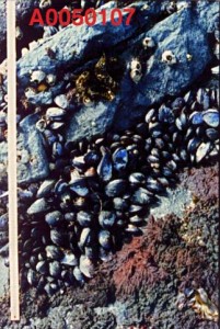 .
.
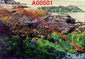
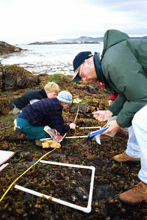
1. For instance from this image from the first transect, A00501, (A0 being the Race Rocks location, 05 being the sample station location and 01 being the first transect at that location, 07 being the seventh quadrat from the top of the intertidal zone. ). Quadrat 07 looks like this. By clicking on this icon you will see this one sample of the actual photo from the transect file.
2. If we want to define the space that the mussels occupy in this quadrat, we have to measure the percent of the quadrat that they are covering. This could be done simply by cutting out a piece of acetate that has been made by xeroxing a piece of graph paper and overlaying it on the screen.
3. A more precise way of doing this is by using an Imaging program to help analyse different aspects of the photograph. Download this image by clicking on the full size image then pressing and holding the right mouse button on a PC or pressing and holding the mouse of a Macintosh . Note that the mussels occupy a portion of this quadrat, a meter stick on the left side gives you the size of the quadrat.
4. CONVERTING THE IMAGES:
Since the above image is in a .JPG format , it has to be converted to a .PICT format for image processing. Do this with a graphic processing program .
5. Using GifConverter: Open the .jpg file obove that you have downloaded. Save it as a .PICT file. This is the format that is necessary to use in the next stage of the process, using NIH Image to measure features of the picture.
6. If you do not have a copy of the freeware NIH IMAGE. Download it from this site. (Both Mac and PC versions are available)
7. INSTRUCTIONS FOR NIH IMAGE: See this file :
Measurement of Surface Area Using “NIH IMAGE”
Also there may now be other software that is easier to use for measuring surface area coverage if one does a google search.
UPDATE: Also from NIH .. ImageJ. http://wsr.imagej.net/distros/
Calibration:
a) To calibrate the image in terms of real units: Use the straight line tool on the left panel, and draw it the length of the meter stick.
b) Use the pull-down menu called “Analyze”; go to “Set scale” . Change the units to centimeters, and “known distance” to 100.00, then hit “OK”.
c) To compute area: From “Tools” menu, select the heart-shaped tool. Outline the total area occupied by mussels. Click on “Analyze options” ; be sure the area box is selected). Press “OK”. From tool bar, select “Analyze”, “Measure”, “Analyze”, “Show results”. A table appears with the area of mussel coverage (in cm2). To compute % area occupied by mussels, measure the total quadrat area with the above procedure except use the rectangle measurement tool to outline the entire quadrat box.
8. DOWNLOADING THE TRANSECT IMAGES: Now, repeat this procedure with all the quadrats in the belt transect strip that contain mussels, you will also have to copy down the elevation found at the base of each quadrat as well..
Go to one of the transect files.
See Transect A0050101
See Transect A0050102
See Transect A0050103
9. Select one of the transects, and download the clips.
 10. USING A SPREADSHEET
Now we have to enter the data into an EXCEL or other suitable spreadsheet.. We will give the detailed instructions for EXCEL.
Enter data in column format (each column is a separate variable).
Calculate:
(a) % area covered by mussels for each transect (area covered by mussels/total area)
(b) percent slope: distance in perpendicular height (elevation change between adjacent quadrats divided by the linear distance (one meter) .
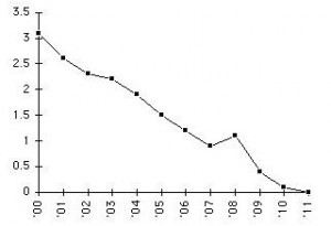
To evaluate terrain gradient for each transect (that is, the steepness of the intertidal shoreline), you can graph the relationship between elevation and slope .
 See this example .Here is a sample of the mussel distribution data as it appears on this spread sheet
 PLOTTING IN 3D
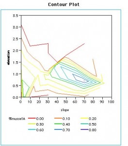
The goal of the analysis is to both describe and predict the environmental space that mussels must occupy in order to survive. The first step in the formal process is a graphical description of the environmental space actually occupied by the animals. In this example, the environmental space is the two dimensional space defined by the variables elevation and slope; the biotic “response” is the percent area occupied by mussels.We imported the variables X1 = “elevation”, X2 = “slope”, Y = “% mussel area” into a standard 3D graphics package (e.g. JMP-Contour Plot). The resulting graph gives the contour plots of mussel density as a function of the 2 environmental variables. Interpretation is similar to reading contour lines on an ordinary topographical map. Note that the “optimum” area for mussel settlement is a range of values for elevation and slope rather than a single point.
This file on Ecological Niche Models was developed by Penny Reynolds, Richard Rosecrance and Garry Fletcher at the Bioquest Consortium Workshop, on WHAT CAN WE LEARN FROM CONTEMPORARY MATHEMATICS REFORM? June 21-29, 1997. Beloit, Wisconsin. It was supported by a grant from the Howard Hughes Medical Institute to : The BioQuest Curriculum Consortium
1. Other websites on Photo transects :
Getting to the bottom of things
http://sango.churashima.okinawa/monitoring_en/cpc.html
 Return to the Contents page for Environmental modelling with Transects..
6 month fouling records
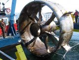
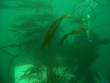
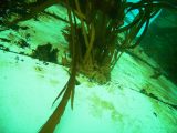
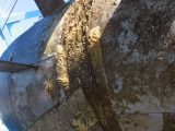
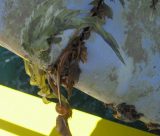
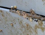
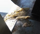
A week before raising the turbine in April 2007, the outer Nereocystis growth was removed by the Pearson College Divers. Since the top of the turbine is in a water depth averaging 10 metres it is shallow enough for the brown Macroalgae to take foothold and within a few weeks it would have reached the surface. This algae can atttach to a solid substrate within the top 12 metres of water at Race Rocks.
- In April, 2007, the turbine was pulled up for inspection and possible refit of bearings.
- Growth of this macroalgae starts in March and had already reached several metres in height
- The kelp holdfasts were attached to the outer cowling on irregularities on the surface.
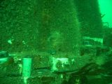
- A felt-like growth of algae and hydroids has already covered the flange below the turbine.
- It gave us an opportunity to examine the distribution of the species and level of growth of the fouling organisms.
- It also provided evidence of which materials are best in repelling growth
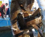
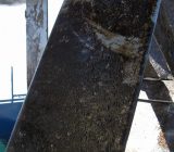
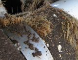
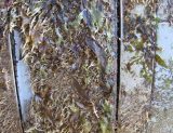
- . Many areas were completely covered with encrustations of diatoms or hydroids. This is one of the blades of the turbine.
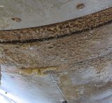
- A scrape on the blade shows the thickness of the diatoms.
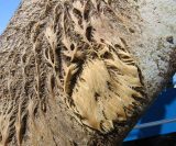
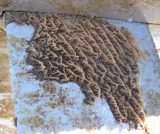
- These hydroids are likely the species Plumularia lagenifera
- All hydroids were of the order Leptothecatae with no Anthoathecatae observable.
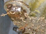
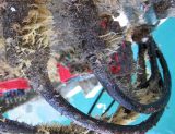
- As in other instances we have experienced when there was long term deployment of instruments at Race Rocks, colonies of skeleton shrimp, shown here, cover some surfaces, and cling to the hydroid colonies.
- Skeleton shrimp (Caprella laeviuscula) hang from their rear appendages in this enlarged photo of a bolt head.
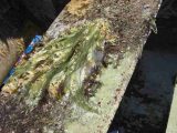
- Various species of red and brown algae ( Laminaria sp ) starting to grow, with more skeleton shrimp scattered throughout
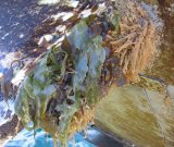
- The turbine was too deep for the growth of green algae. These brown algae, Desmarestia sp. were attached to a blade. They appear green since they have been drying out for some time and the acids in the lamina tend to speed deterioration of pigment
- A few small bull kelp, (Nereocystis leutkeana) have anchored to the structure. This could provide problems for future entanglement if these kelp thrive on the structure.
- A mixed population of some red and brown algaes.
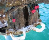
- In the areas underneath the structure where the cables attach, a good amount of protection is available thus encouraging the attachment of the fouling species.
- A 1 cm diameter barnacle has attached to this part of the structure. Note also skeleton shrimp.
- It demonstrated the problem of having any small crevice or location where organisms could establish a foothold on the structure.
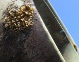
- Hydroid clump on the underside of the cowling.
- Colonial Tunicates, the gelatinous yellow mass along one seam, have started to colonize in this area.
- Diatoms coat many of the exposed surfaces. They are usually the precursor to futire invertebrate growth..
Thanks to Russell Stothers of Clean Current and the Pearson College Divers for these images.
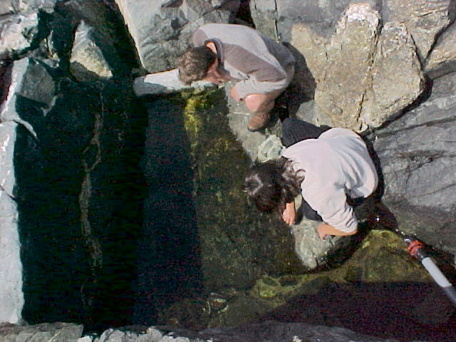
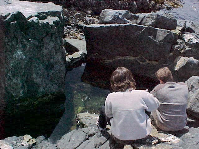
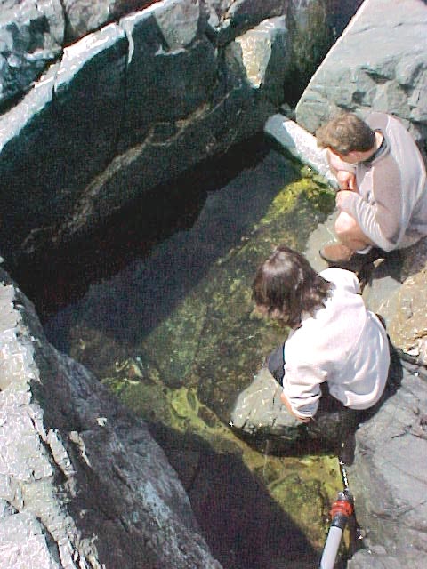
Artificial Tidepool #13 peg #5
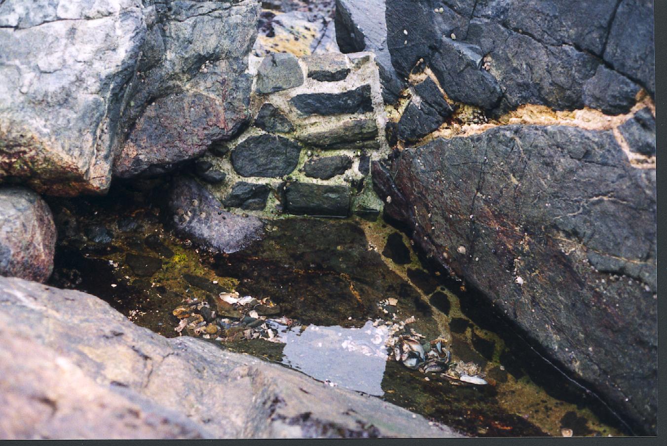
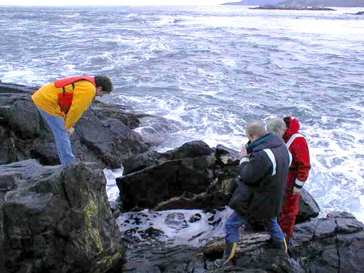
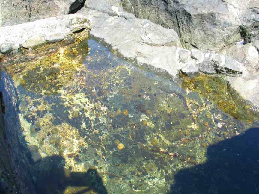
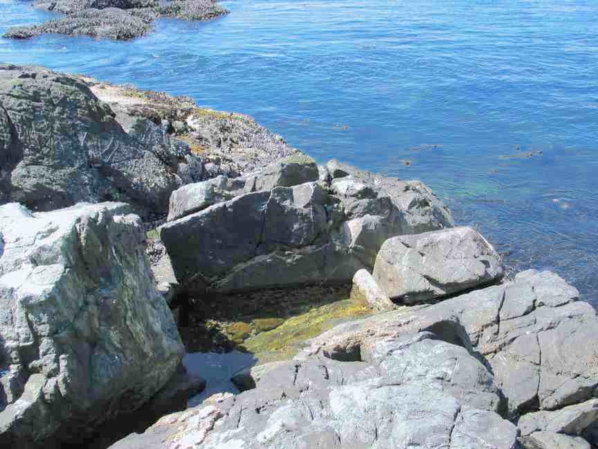
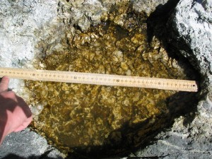
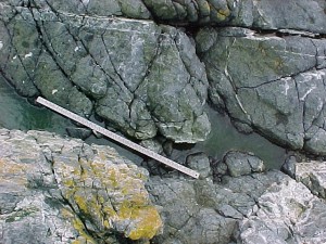
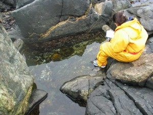
This artificial pool was made under permit from BC Parks by Mike Slater and Garry Fletcher in June, 1999. It is part of a long range succession study.
See also below for “AFTER the HURRICANE”
- Observing the action of water as a surge fills the pool.
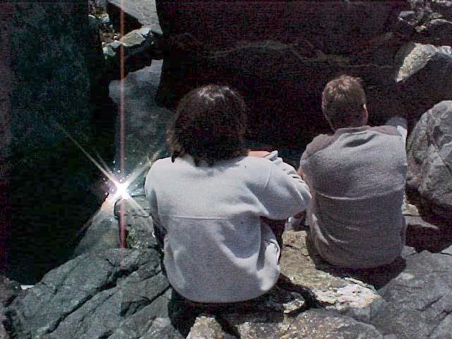
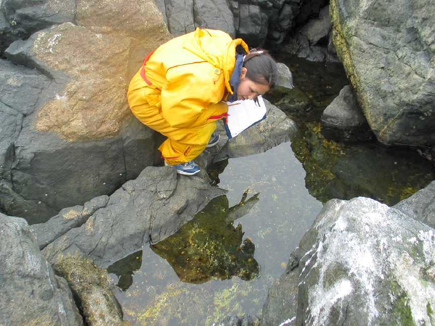
- Students surveying the pool.
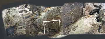
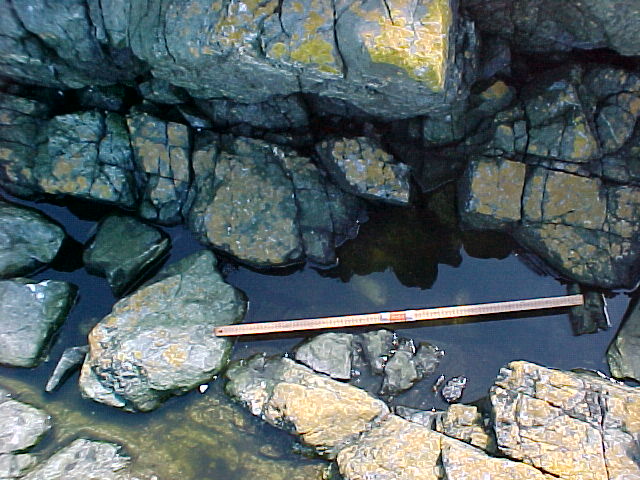
- A panorama of the pool before water filled it. The white quadrat is 50cm on each side.
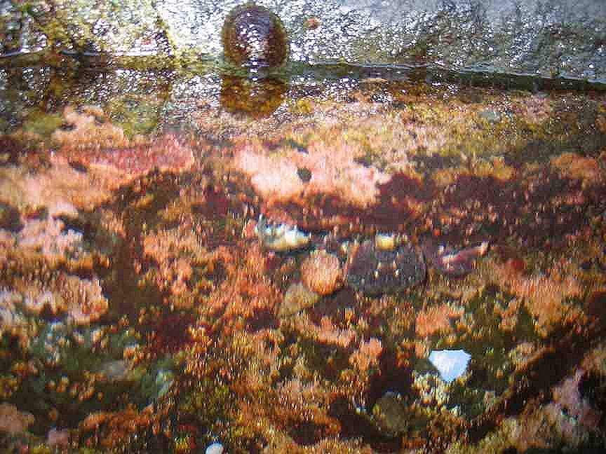
- In May of 2005 Kinwa sees that the tidepool has a number of invertebrate inhabitants
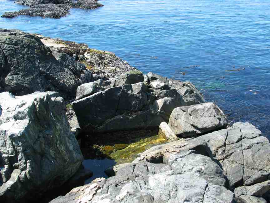
- A view from above looking seaward.
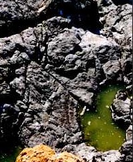
- June 5 2005A view of the whole pool from above.
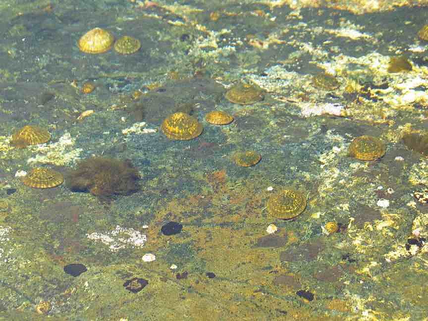
- Limpets graze on the algal growth on the flat bottom
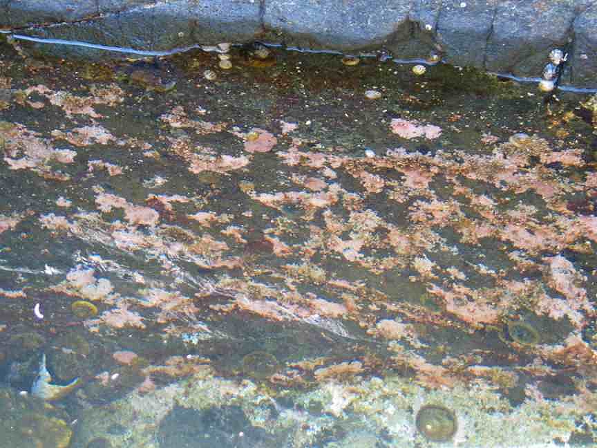
- On the West side, the pink encrusting algae Lithothamnion grow
- The purple shore crab hangs onto a ledge on the West side. just below the surface.
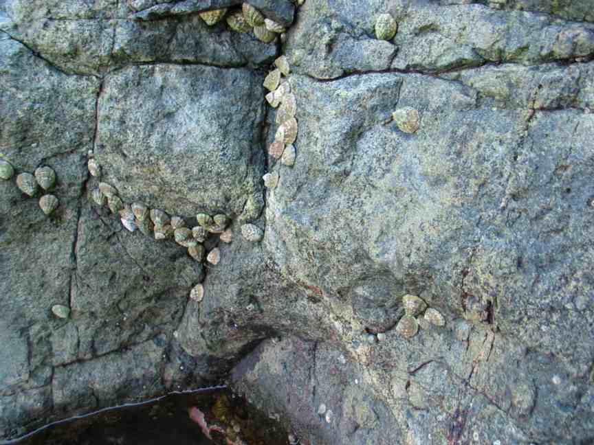
- On the South wall finger limpets are in their same location as before the pool was built.
- The North and West side of the pool
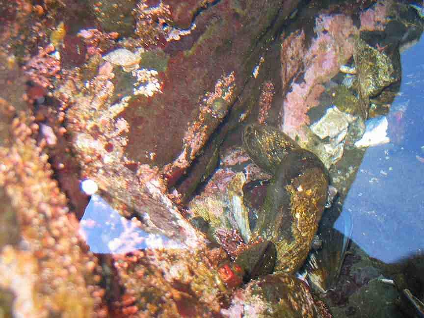
- Californianus mussels
- On the bottom corner agroup of Californianus mussels has established a foothold.
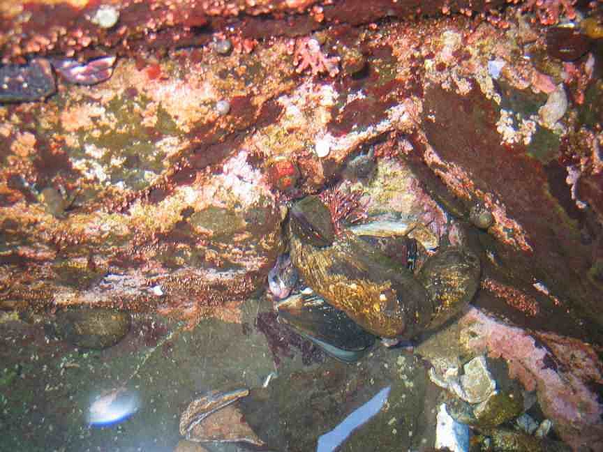
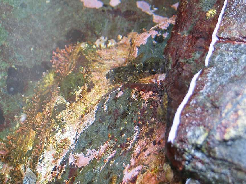
- A tidepool sculpin sticks his head out from under the ledge beside the rock-concrete wall
AFTER THE HURRICANE OF DECEMBER 15, 2006 (newspaper item)
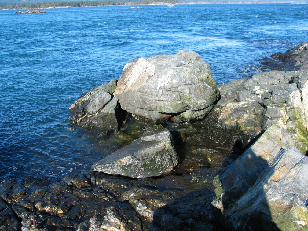
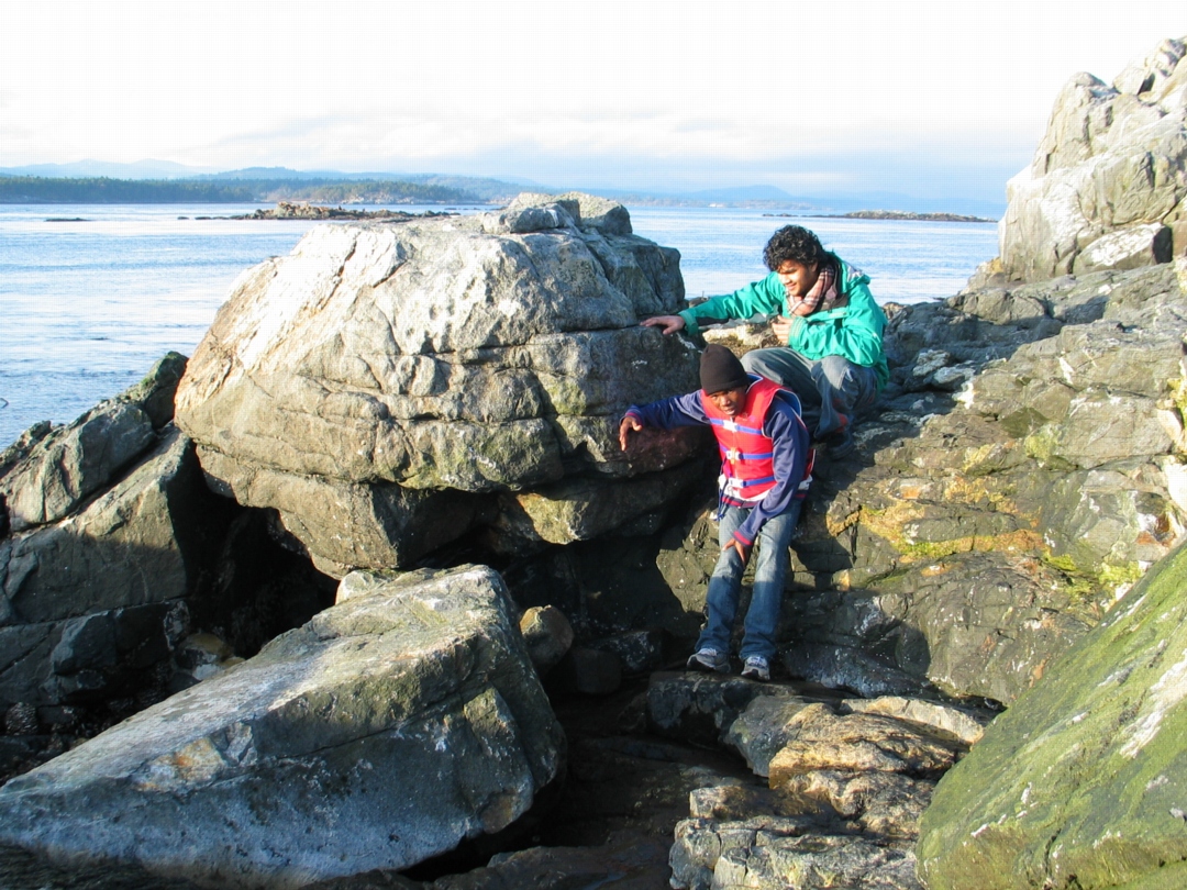
- Before the hurrricane, viewed from the north side, it appeared as above. The large rock on the left side of the picture was moved….
- .and after the huuricane, it sits on top of the tidepool.and completly covers the pool
- Viewed from the South side,
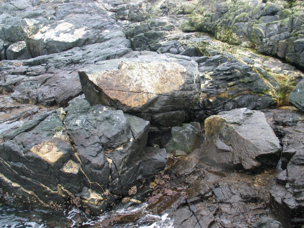
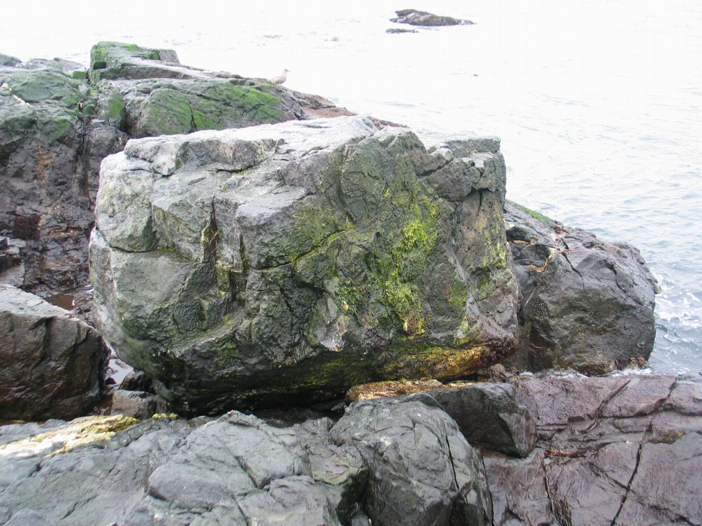
- Looking at the South West corner of it. The large square rock that used to be on the ocean side of the boulder is now gone completely.
- This is the space previously occupied by the smaller seaward boulder.
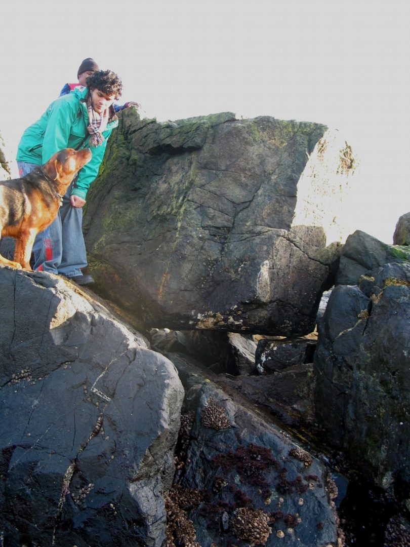
- The same view below the large boulder, with students Mujahed,Anitesh and Kip.
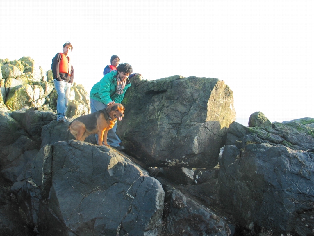
- Anitesh and Kip stand where the boulder once was sitting,
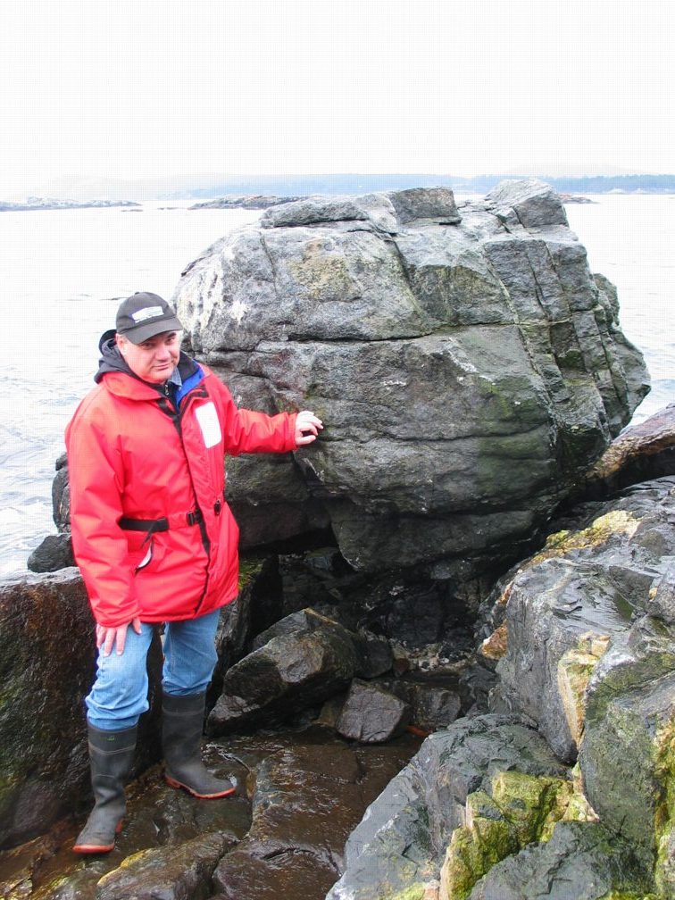
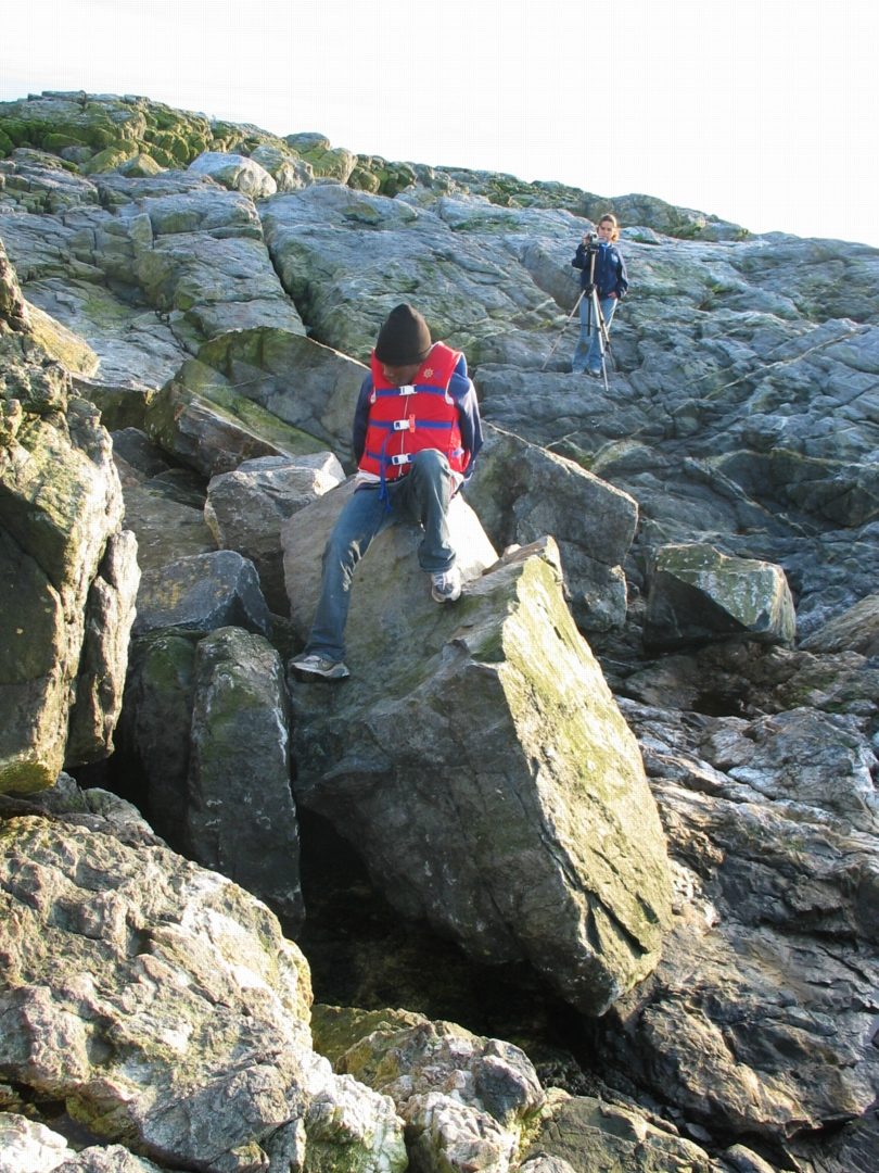
- Jack Knox stands on the east side of the rock in the middle of where it where it used to be sitting.
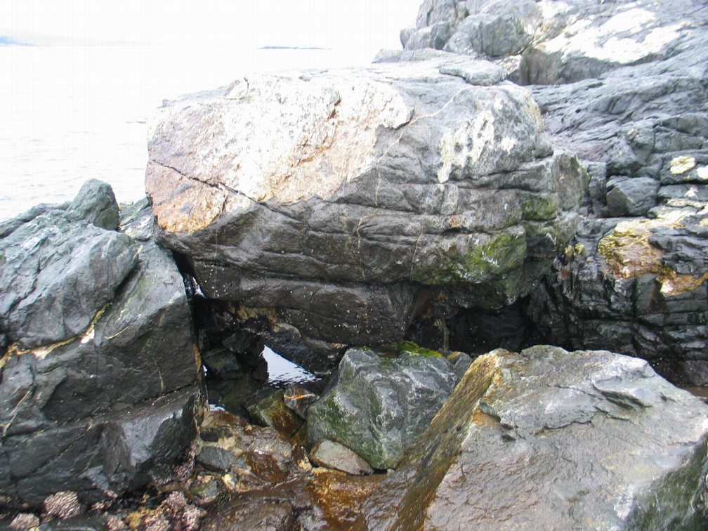
- The boulder perches directly over the pool resting against the concrete dam built on the west side of the pool and a small rock directly underneath.
- the moved boulder
- The stone wall we had built on the south side is still standing..The tidepool now, in under the boulder. It is also filled with large rock
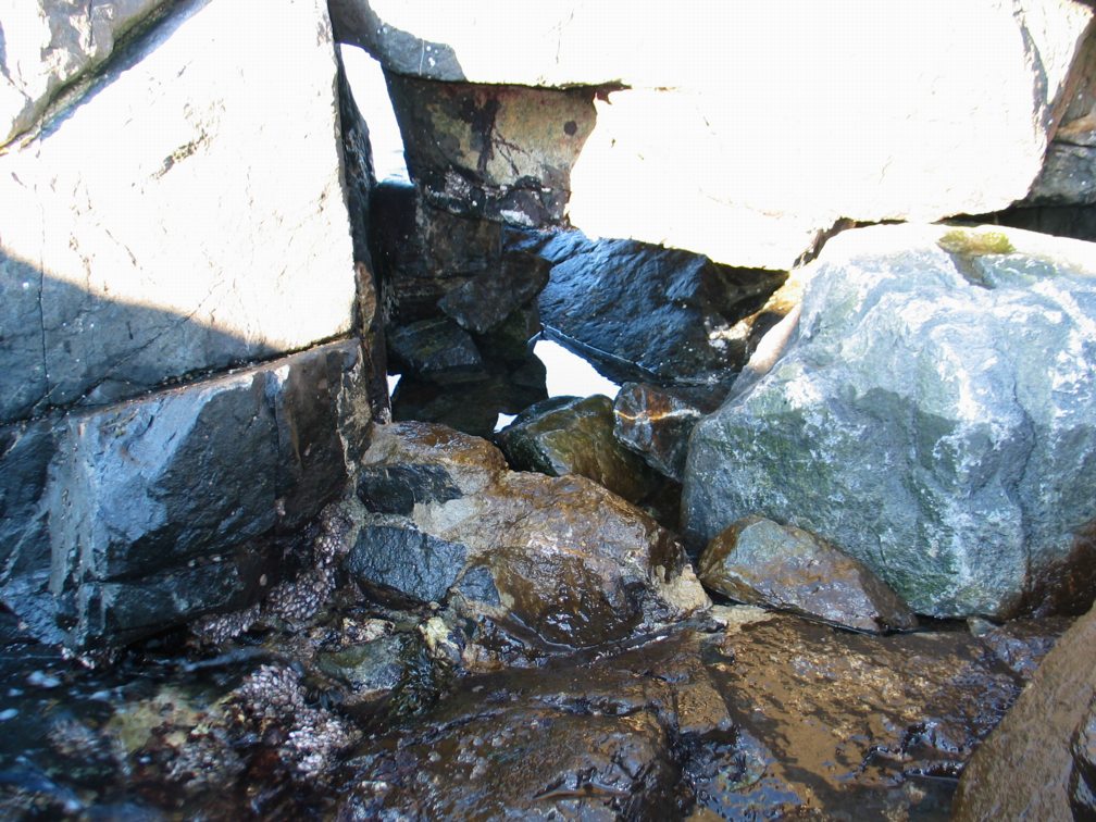
- These large boulders up the shore from the tidepool have also moved 2 to 3 meters
Sea Water Temperatures at Race Rocks
 From From1921 until 1997 daily records of Seawater Temperature and Salinity were manually taken at Race Rocks by the Lightkeepers and assistants. In 1997 the station was automated and Lester Pearson College took over the hiring of the Lightkeeper Mike Slater and his wife Carol as Guardians for the Ecological Reserve / Marine Protected Area. They maintained the daily sea temp and salinity records until their retirement in 2009. The records have been submitted monthly to the Institute of Ocean Sciences, thus continuing this important long term record. See the Decade Comparisons:Sea Surface Temperature at Race Rocks- 1921-1930 and 1995-2005
|
|
Garry gives a good demonstration of when one should avoid taking seawater temperatures!~ (Photo by Barry Herring Feb 2009)
|
|
SEA TEMPERATURE 1921 to 2008 FROM British Columbia Lightstation Sea-Surface Temperature and Salinity Data (Pacific), 1914-presentAlso http://www.pac.dfo-mpo.gc.ca/science/oceans/data-donnees/lighthouses-phares/data/racerockday.txt |
| Refer to the File “Temperature Changes Through Time for an Educational exercise on Sea water Temperature changes. |
| OCEAN WARMING: The long-term Sea temperature record at Race Rocks has been pointed out as one of the pieces of evidence that has accumulated on global warming. Terry Glavin, in reviewing the book The Weather Makers by Tim Flannery ( Harper Collins Publishers, 2006) says :” The Pacific Ocean itself is getting warmer. Measurements at the Race Rocks lighthouse near Victoria show an average rise in temperature of 1°C since 1921, which doesn’t sound like much until you remember that its only 10°C in the other direction that separates us from the deep freeze of the Ice Age. The ocean, absorbing increasing volumes of carbon dioxide, is becoming more acidic too, inhibiting the production of plankton, the basis of all life in the sea.”The rest of the article may be seen at http://www.straight.com/content.cfm?id=17132 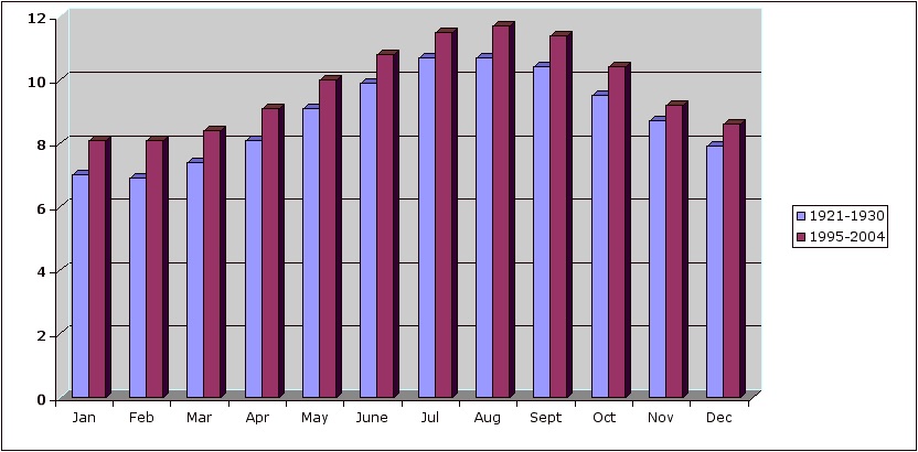 See this file for our own analysis which supports this statement: See this file for our own analysis which supports this statement: |
page 21 State of the Pacific Ocean 2005 context.http://www.pac.dfo-mpo.gc.ca/sci/psarc/OSRs/StateofOceans2005fnl.pdfTwo references are made to Race Rocks Sea Temperature data. page 6 and page 31 |
| State of the Pacific Ocean , 2006 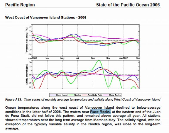 state of the pacific ocean 2006,page 36 ” Ocean Temperatures along the west coast of Vancouver island declined to below average conditions in the latter half of 2006. The waters of race Rocks …did not follow this pattern, and remained above average all year.” |
| RESPONSE OF ORGANISMS TO SEAWATER TEMPERATURES: |
| The seawater in the Strait of Juan de Fuca has a very narrow variation in temperature range. It is important to understand about Heat Capacity, as it is partly due to this ability of water to warm up slowly and cool off slowly that the climate of Vancouver Island and the lower mainland of British Columbia has the mildest weather in Canada. |
| Heat capacity is the ratio of the heat energy absorbed to the rise in temperature. Objects with high heat capacity, such as water, require a great amount of heat energy to change temperature. Materials with low heat capacities, such as air, easily change temperature with small amounts of heat energy. These
Other ideas to be developed here: 2. 3. 4. |
 |
Dr.
Kate Edwards of the University of Washington School of Oceanography is doing research on the sea temperatures of the Strait of Juan de Fuca. (click on image to left).She maintains web pages at: Strait of Juan de Fuca page: http://www.ocean.washington.edu/~kate West Coast headlands page: http://www-ccs.ucsd.edu/~kate |
| Jan Newton is at the Washington state Department of Ecology and is interested in how the Straits affect Puget Sound. She has organized the “Joint Effort to Monitor the Straits,” which regularly sample the three stations south of San Juan Island in the map at http://www.ecy.wa.gov/apps/eap/marinewq/mwdataset.asp . Click on the Station Group Puget Sound, and the Selected Station – Juan de Fuca. |
|
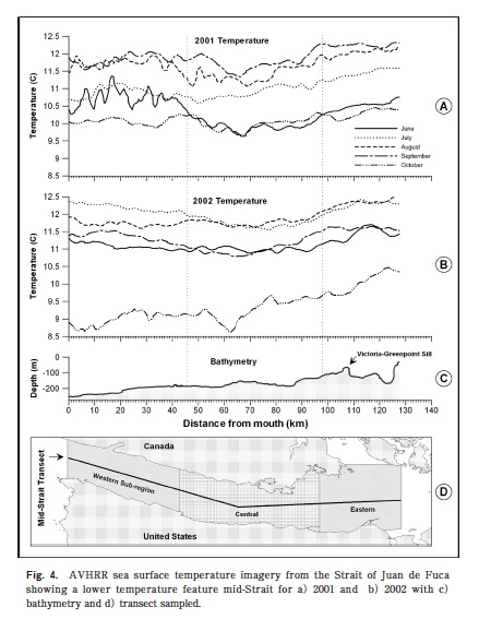 This paper references Strait of Juan de Fuca Temperatures |
| Educational Exercises Using Data From Race Rocks – Excel and Statistics |
Tidepool Index:
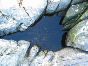
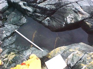
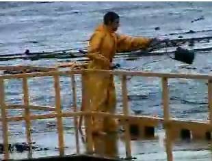
These pools are located 0n the West side of Great Race Rocks. They are located at slightly different elevations resulting in different abiotic factors in the pools and different life forms in the pools as well. Our students brave the elements to get some measurements in this video
| Tidepool 11: No File for this pool | |
ph as an abiotic factor
| The effects of pH on the distribution of organisms at Race Rocks. Useful Links:
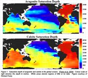
“Global oceans are becoming more acidic due to increasing carbon dioxide (Orr et al. 2005). Much of the extra CO2 released by burning fossil fuels ends up in the oceans, increasing the dissolved inorganic carbon concentration (DIC). As DIC increases, the relative proportions of carbon species shift (specifically from the carbonate ion to the bicarbonate ion), resulting in an increase in acidity and a decrease in pH (Strum and Morgan, 1981). At present the pH of seawater has decreased by about 0.1 due to oceanic uptake of anthropogenic carbon and is projected to decrease by 0.4 by the year 2050 (Orr et al. 2005). The decrease in pH (and concurrent decrease in carbonate ion) means that organisms that produce calcite and aragonite shells or structures, such as pteropods, corals and shellfish, are threatened (The Royal Society, 2005).” 2. THE EFFECT OF HYDROGEN ION CONCENTRATION UPON THE INDUCTION OF POLARITY IN FUCUS EGGS http://www.jgp.org/cgi/content/abstract/20/3/491 3. THE EFFECT OF ALKALINITY UPON MUTUAL INFLUENCES DETERMINING THE DEVELOPMENTAL AXIS IN FUCUS EGGS 1. When two eggs of Fucus furcatus develop in the dark within 0.3-4 egg diameters of each other, the point of rhizoid origin and the developmental axis are influenced by the presence of the neighbor. http://www.biolbull.org/cgi/content/abstract/78/3/407 4. Discovering the Effects of CO2Levels on Marine Life and Global Climate In recent months, the media have begun to focus on another effect of rising atmospheric CO2 concentrations: the effect of increasing CO2 levels on marine life. The oceans absorb 22 million tons of carbon dioxide every day, writes Richard Feely, a scientist with the National Oceanic and Atmospheric Administration (NOAA) in a 2006 science brief, “Carbon Dioxide and Our Ocean Legacy” (100 KB PDF). Although this absorption is said to significantly reduce atmospheric greenhouse-gas levels, some scientists have observed that such an excess of CO2 may be altering the chemistry and biology of the world’s oceans.By Kate Bradshaw 5. Dropping pH in the Oceans Causing a Rising Tide of Alarm http://www.thew2o.net/archive_new.html?id=28 6. Researchers report on possible biological effects .http://www.mbari.org/news/news_releases/2001/oct12_seibel.html 7. Bush’s CO2 Dumping Plan Could Devastate Sea Life http://www.scienceagogo.com/news/20031019174538data_trunc_sys.shtml 8. SEAKEEPERS PROVIDING KEY DATA ON OCEAN ACIDIFICATION AFFECT ON GLOBAL WARMING http://www.seakeepers.org/featured-ocean-acidification.php 9. Also a general index at: https://search.usa.gov/search?affiliate=usgswebarchive&query=ph |
| See also our file on Ocean Acidification in 4.2 The Importance of pH. |
Adopt an Ecosystem
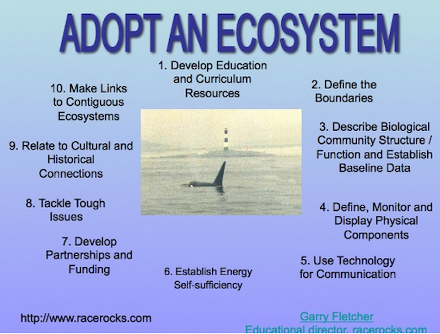 BACKGROUND: “Adopt an Ecosystem” involves using the internet as a means to get individuals and groups in other communities: provincial, state, national and international, involved in collaborating with others, and providing an educational resource while ensuring the stewardship of their own local ecological resources.
OUTLINE WITH POWER POINT PRESENTATION:
This 10 step outline presents the basic model of how to go about setting up an Adopt an Ecosystem Project in your school or organization.
THE PROCESS:
We are urging individuals, school groups and service groups in communities to establish internet files on a local natural area which they are able to document easily at a number of levels of scientific sophistication. This natural area may be a small corner of a school yard, a piece of coastline, a local stream or pond, or it could be an established ecological reserve or park. Valuable long-term baselines can be established with students of each year or individuals leaving a “digital legacy’ or a permanent on-line record which is available for other classes to make additions and updates in the future.
THE IMPORTANCE OF THE “PROCESS”
By involving individuals in the documentation and monitoring of their adopted ecosystem, a sense of “ownership” of one’s ecosystems and responsibility for their stewardship is experienced. In addition participants are encouraged to use technology to assist in the accumulation of valuable long-term ecological information which can serve as baselines for environmental impact decisions in the area, and as a valuable baseline on the area’s biodiversity.
OBJECTIVES: (The teacher and class may decide on setting their goals for this project, using only a limited number of the suggested activities.) After doing this assignment, students will be able to:
a) Design a plan and procedure for the creation of a local : “Adopted Ecosystem”
b) Use field methods involving quantification to document the chosen ecosystem with a baseline inventory.
c) Use a Spreadsheet program for the analysis and recording of locally collected data.
d) Set up a weather station for collection of weather data.
e) Construct a species list and/or taxonomy of the local organisms in the “Adopted Ecosystem”.
f. iNaturalist contributions Recently I opened an account on iNaturalist.com . I have been able to add many pictures of species taken around the Metchosin coast, as well as other locations. https://www.inaturalist.org/observations/garryf
It is a great idea to contribute to iNaturalist so by opening a free account on iNaturalist.com it is a good way to do establish a baseline for organisms in your ecosystem and get professional assistance from experts for identification of species. for instance for the biodiversity project the following entries are recorded by various individuals, https://www.inaturalist.org/projects/metchosin-biodiversity
f) Setup a website dedicated to the collection of resources relating to your locally adopted ecosystem.
g) Outline the Ecosystem Services and the value of the Natural Capital of your adopted Ecosystem.
PROCEDURE:. Identify the area and describe the ecological features that make the area unique, important or just representative of other surrounding ecosystems. Also indicate what your group intends to do with it.
2. You may indicate time lines for your goals, and even designate responsibilities to different group members in order to help you plan your strategy.
3. Establish a good “baseline inventory ” of what is there presently. Many ecological techniques are available to quantify organisms and their distribution. You may use our Transect Files as an example.
4. Establish a class project to provide a taxonomy of the species of your local ecosystem.
5. Include dated maps, databases, taxonomic inventories, checklists, photographs, videos or drawings to document your site. Open a project on iNaturalist.com that enables you to enter photos of species and have experts help in making identifications
6. Begin monitoring the site for aspects of its structure and function. For structure: what living things are there, how they are distributed, what relationships or biotic associations exist. Also, the structure includes physical factors such as temperature, salinity, etc. –start gathering long term data, enter it into a database (such as excel), and save it to the internet site so that others can download and manipulate the data.
7.Download Google Earth and make a 3 dimensional image of the area with your ecosystem.
8. Search for historical and other recent maps or charts of your area. Include these as part of the information recorded.
9. If you have access to your own internet site, assemble the information on the site, let us know its location and we will provide a link to your site from racerocks.ca.
10. Establish a Project to list and value the Ecosystem Services and Natural Capital of your ecosystem. In recent years, we have started to acknowledge that “ecosystem services ” are something to which we must start paying attention as to fail to do so leads to a decline in quality of life:
This file explores that idea further and invites you to contribute to a new project : Defining the Ecosystem Services of Race Rocks. By looking at the model of such services developed for Race Rocks, you might also get an idea how you could choose a part of your own local ecosystem and do a similar analysis.
11. In the fall of 2005 we installed a Davis Weather Instrument at Race Rocks for real time monitoring of a number of meteorological events.
From this environmental data index page, you can see how we are developing pages for each environmental abiotic factor and interpreting how that factor is important in the ecosystems of Race Rocks. Many schools already have weather stations installed. Here are some examples from the Victoria area:
Send inquiries to: Garry Fletcher
Archives: Videos of Science and Education at Race Rocks.
The students of Lester Pearson College are frequently taken to Race Rocks for educational field labs. Pearson College has, since automation in 1997, paid for the staffing and upkeep of the island. These videos portray some of the exercises that are done throughout the year on the island. The college biology and environmental systems classes, students on special projects, and outside researchers make extensive use of the facilities. In addition several videos portray the physical factors that help to make Race Rocks an unusual ecosystem.
Facilities on the Island and the MPA.
 |
 |
 |
|
| Installation of Composting Toilets at Race Rocks | The future of alternate energy at Race Rocks. Interview with Taco Niet, Masters student at the University of Victoria (June 2001) |
Race Rocks is officially declared a Marine Protected Area by Canada’s Ocean’s Minister Herb Dhaliwal and British Columbia’s Environment Minister Joan Sawicki. Also see the MPA day File. |
Underwater Research
at Race Rocks
 |
 |
 |
 |
| Abalone tagging at Race Rocks with Pearson College graduate Jim Palardy | A dive with Dr. Scott Wallace for the Discovery Channel, May 7, 2000 |
Alberto Lindner of Brazil visits Race Rocks for research on the Hydrocoral Allopora | Dr. Gitai Yahel and research on Ecology of Suspension Feeders |
Physical Factors and their Effects on Race Rocks
 |
 |
 |
 |
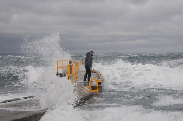
| Tidal Level Variation at Race Rocks | Surge Channel and Surge as an Abiotic Factor | The Flood Current at Race Rocks | Wind Storm at Race Rocks |


