Archives: Videos of Science and Education at Race Rocks.

The students of Lester Pearson College are frequently taken to Race Rocks for educational field labs. Pearson College has, since automation in 1997, paid for the staffing and upkeep of the island. These videos portray some of the exercises that are done throughout the year on the island. The college biology and environmental systems classes, students on special projects, and outside researchers make extensive use of the facilities. In addition several videos portray the physical factors that help to make Race Rocks an unusual ecosystem.

Video by AZIZ, 2016


 Laura Verhegge’s first year environmental systems class doing their end of term exam at Race Rocks, May 2002.  A session with the biology class by the high tidepools at Race Rocks.  The Environmental Systems Field Exam, May 2000
 April, 2000: Environmental systems classes of LBPC  in  tidepool study on the W.side of Great R.R. This is part of the class report .
Outpost- A film on the educational activities at Race Rocks 1997 Some Intertidal Discussions- Johan Ashuvud week June 2004 Underwater Belt Transect survey. Laura Verhegge and students of Lester B.Pearson College
School Visits
June 2002 field trip: for a live webcast of the grade six students of Westmont school A school visit by Journey elementary school in June to Race Rocks Second day of students’ visit in June. Students are shown how the cameras function at racerocks. i
Pearson College Students assist as
Ecoguardians Daily Life
Race Rocks Tour:English Version
Arabic Version
German Version
Daily Duties For Assistants to the
MPA Guardian
Daily life of the students staying for a project at Race Rocks.

Facilities on the Island and the  MPA.
 Installation of Composting Toilets at Race Rocks  The future of alternate energy at Race Rocks.
Interview with Taco Niet, Masters student at the University of Victoria
(June 2001)
 Race Rocks is officially declared a Marine Protected Area by Canada’s Ocean’s Minister Herb Dhaliwal and British Columbia’s Environment Minister Joan Sawicki.
Also see the MPA day File.

Underwater Research
at Race Rocks

 Abalone tagging at Race Rocks with Pearson College graduate Jim Palardy  A dive with Dr. Scott Wallace for the Discovery Channel,
May 7, 2000
 Alberto Lindner of Brazil visits Race Rocks for research on the Hydrocoral Allopora  Dr. Gitai Yahel and research on Ecology of Suspension Feeders

Physical Factors and their Effects on Race Rocks

 Tidal Level Variation at Race Rocks  Surge Channel and Surge as an Abiotic Factor  The Flood Current at Race Rocks  Wind Storm at Race Rocks

Salinity as an Abiotic Factor

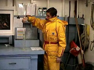
Jeremias tests the salinity using a hydrometer. This manual method has been used at Race Rocks from 1935 until more recent years when a digital salinometer has been used.


For monthly records of Salinity refer to :

https://www.racerocks.ca/?s=Salinity&submit=Search


“During our project week at Race Rocks, Mike Slater, the Race Rocks Marine Protected Area Guardian asked us if we could make a video explaining the daily duties necessary to maintain the facility. Students who are relieving on the island during Mike’s absence will be able to use this data as a guide for performing their duties, as well as providing a useful information resource for students visiting the island.

These duties include two daily engine checks, a salinity check one hour before high tide, and keeping a record of the days weather, as well as explaining the functions and instructions for testing machinery located on the island.”

ABIOTIC EFFECTS OF SALINITY ON ORGANISMS

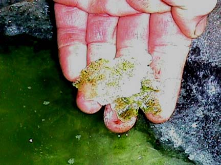
Organisms which live in Tidepools have to withstand changing salinities which may range from 0 parts per thousand to over 100 parts per thousand. Here is an example of an algae that in the summer lives in concentrated brine of the evaporated tidepool number 7.


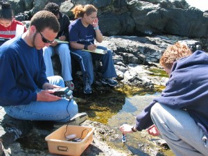
Rob measures salinity with the salinometer in tidepool Number 4..This file shows the results that one class in environmental systems got when measuring the salinities of tidepools. Note there can be quite a variation in both temperature and salinity, depending on the elevation of the pool and therefore the frequency of flooding from the ocean.

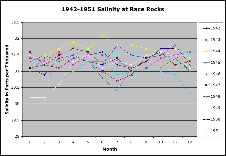
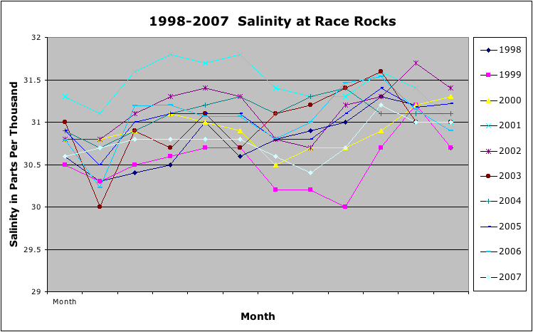
Mean Monthly Sea Surface Salinity at Race Rocks-1936 to present .

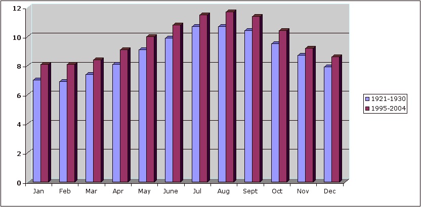
Two decades of mean monthly Salinity records are compared in the following investigation.

Salinity Comparisons for 2 Decades
There are a number of interesting features of the two decades almost 50 years apart.

Some open-ended questions that you may wish to pursue:

  1. How do the individual months compare?
  2. Is there any evidence of a trend that distinguishes the earlier decade from the most recent one?
  3. Is there any evidence of a trend that distinguishes one period of the year from another?
  4. What could be the cause of any observable trends?
  5. Does geographic location of Race Rocks provide an answer to any findings?
  6. See the work done on comparing sea temperature from two decades for some other ideas.
  7. What would the graphs look like if you took the means of each month from the two decades and plotted them ?

You may also see the the raw data used to make the graphs in the two tables below. It may be useful in this format to clip and paste into an EXCEL workbook for further analysis. If you come up with any other interesting analysis of the data from this exercise or from looking at the complete data archive. We would be interested in carrying it attached to this page.

Raw Data 1942 1943 1944 1945 1946 1947 1948 1949 1950 1951
Jan. 31.1 31.4 31.5 31.3 31.1 31.6 31 31.3 31.1 30.2
Feb. 30.9 31.3 31.5 31.2 31.2 31.2 31.4 31.5 31.1 30.2
Mar. 31.4 31.6 31.7 31.5 31.1 31.5 31.4 31.3 30.7 30.6
Apr. 31.5 31.2 31.9 31.5 31.4 31.7 31.5 31.5 31 31.3
May 31.5 31.5 31.7 31.7 31.3 31.6 31.3 31.3 31.3 31.5
June 31.6 31.5 32.1 31.6 31 31.2 30.8 31.2 31.3 31.1
July 31.2 31.3 31.8 31.5 30.7 31.4 30.4 31.8 30.9 31.3
Aug. 31.1 31.1 31.8 31.5 30.9 31 31.1 31.5 31 31.2
Sept. 31.3 31.1 31.7 31.6 31.4 31.4 31.1 31.4 31.1 31.5
Oct. 31.7 31.4 31.6 31.8 31.5 31.6 31.1 31.5 31 31.6
Nov 31.7 31.5 31.7 31.8 31.8 31.2 31.4 31.5 30.9 31.5
Dec 31.4 31.6 31.4 31.5 31.2 31.3 31 31 30.3 31.1
1998 1999 2000 2001 2002 2003 2004 2005 2006 2007
Jan. 30.6 30.5 30.8 31.3 30.8 31 30.9 30.9 30.79 30.6
Feb. 30.3 30.3 30.8 31.1 30.8 30 30.7 30.5 30.23 30.7
Mar. 30.4 30.5 30.9 31.6 31.1 30.9 30.9 31 31.19 30.8
Apr. 30.5 30.6 31.1 31.8 31.3 30.7 31.1 31.1 31.2 30.8
May 31 30.7 31 31.7 31.4 31.1 31.2 31.1 31.07 30.8
June 30.6 30.7 30.9 31.8 31.3 30.7 31.3 31.1 31.07 30.8
July 30.8 30.2 30.5 31.4 30.8 31.1 31.1 30.8 30.81 30.6
Aug. 30.9 30.2 30.7 31.3 30.7 31.2 31.3 30.8 31 30.4
Sept. 31 30 30.7 31.3 31.2 31.4 31.4 31.1 31.46 30.7
Oct. 31.3 30.7 30.9 31.6 31.3 31.6 31.1 31.4 31.54 31.2
Nov. 31.2 31.2 31.2 31.4 31.7 31 31.1 31.18 31.15 31
Dec. 30.7 30.7 31.3 31 31.4 31 31.1 31.22 30.9 31

Daily Air Temperature Data -1998-2005: Race Rocks Ecological Reserve


I am working at restoring the following links which were removed when Telus dropped a server unexpectedly which we had been using at racerocks.com .. If you wish to access this data before i get the links updated ,you may contact me at email :garryf  then use the at sign gmail dot com

October 1984 to February 1997 daily weather records submitted to Environment Canada Meteorological Service by the light keepers at Race Rocks.

Be sure to do a Customized Search for
“Race Rocks Lightstation” to find this archive.

I think previous records exist so I am trying to get them from the Canadian Meteorlogical Service.

AIR DATA, JANUARY 1998
(missing first three months)

AIR DATA, FEBRUARY 1998

AIR DATA, MARCH 1998


>AIR DATA, APRIL 1998AIR DATA, MAY 1998

AIR DATA, JUNE 1998

AIR DATA, JULY, 1998

AIR DATA, AUGUST, 1998

AIR DATA SEPTEMBER, 1998

AIR DATA OCTOBER, 1998

AIR DATA NOVEMBER, 1998

AIR DATA DECEMBER, 1998


AIR DATA, JANUARY 1999

AIR DATA, FEBRUARY 1999

AIR DATA, MARCH 1999

AIR DATA, APRIL 1999

AIR DATA, MAY 1999

AIR DATA, JUNE 1999

AIR DATA, JULY, 1999

AIR DATA, AUGUST, 1999

AIR DATA SEPTEMBER, 1999

AIR DATA OCTOBER, 1999

AIR DATA NOVEMBER, 1999

AIR DATA DECEMBER, 1999


AIR DATA, JANUARY 2000

AIR DATA, FEBRUARY 2000

AIR DATA, MARCH 2000

AIR DATA, APRIL 2000

AIR DATA, MAY 2000

AIR DATA, JUNE 2000

AIR DATA, JULY, 2000

AIR DATA, AUGUST, 2000

AIR DATA SEPTEMBER, 2000

AIR DATA OCTOBER, 2000

AIR DATA NOVEMBER, 2000

AIR DATA DECEMBER, 2000


AIR DATA, JANUARY 2001

AIR DATA, FEBRUARY 2001

AIR DATA, MARCH 2001

AIR DATA, APRIL 2001

AIR DATA, MAY 2001

AIR DATA, JUNE 2001

AIR DATA, JULY, 2001

AIR DATA, AUGUST, 2001

AIR DATA SEPTEMBER, 2001

AIR DATA OCTOBER, 2001

AIR DATA NOVEMBER, 2001

AIR DATA DECEMBER, 2001


AIR DATA JANUARY, 2002

AIR DATA FEBRUARY, 2002

AIR DATA MARCH, 2002

AIR DATA APRIL, 2002

AIR DATA MAY, 2002

AIR DATA JUNE, 2002

AIR DATA JULY, 2002

AIR DATA AUGUST , 2002

AIR DATA SEPTEMBER , 2002

AIR DATA OCTOBER, 2002

AIR DATA NOVEMBER, 2002

AIR DATA DECEMBER, 2002


AIR DATA JANUARY, 2003

AIR DATA FEBRUARY, 2003

AIR DATA MARCH, 2003

AIR DATA APRIL, 2003

AIR DATA MAY, 2003

AIR DATA JUNE, 2003

AIR DATA JULY, 2003

AIR DATA AUGUST, 2003

AIR DATA SEPTEMBER, 2003

AIR DATA OCTOBER, 2003

AIR DATA NOVEMBER, 2003

AIR DATA DECEMBER, 2003


AIR DATA JANUARY, 2004

AIR DATA FEBRUARY, 2004

AIR DATA MARCH, 2004

AIR DATA APRIL, 2004

AIR DATA MAY, 2004

AIR DATA JUNE, 2004

AIR DATA JULY, 2004

AIR DATA AUGUST , 2004

AIR DATA SEPTEMBER , 2004

AIR DATA OCTOBER, 2004

AIR DATA NOVEMBER, 2004

AIR DATA DECEMBER, 2004


AIR DATA JANUARY, 2005

AIR DATA FEBRUARY, 2005

AIR DATA MARCH, 2005

AIR DATA APRIL, 2005

AIR DATA MAY, 2005

AIR DATA JUNE, 2005

AIR DATA JULY, 2005

AIR DATA AUGUST , 2005

AIR DATA SEPTEMBER, 2005

AIR DATA OCTOBER, 2005

AIR DATA NOVEMBER, 2005

AIR DATA DECEMBER, 2005


From January 2006 on, refer to the air temperature files from the Davis Weather Instrument.

Archived Data for this page has been produced in the EXCEL Files by Mike Slater. It was then converted and saved as html by Garry Fletcher and students of the racerocks.com activity


Directory of OceanQuest Assignment Resources:

Overview: Are you prepared to take on the challenge of OceanQuest? You are expected to be an active participant in helping to build a valuable resource database for a unique sensitive environment.

The basic starting resources you will use come from www.racerocks.ca but our vision for the future is that you may actively develop a set of internet resources for your own unique ecological area.

Link to The OceanQuest GIS With Curriculum Guide
NOTE: The link to the GIS which ran on an outside server arranged by the Open School has been discontinued.. The other curruculum materials are still valid however on this site.
Topic 1 :
BIODIVERSITY

Some of the following files from www. racerocks.ca were used in the building of the OCEANQUEST website.
Lesson: 1. Structure and Function of Ecosystems :
How can we model ecosystems in order to understand how they work ?
Student Activities: Objectives:
Procedure :
1. Introduction
2. Horizontal distribution

  • Objectives:
    Procedure:

    • 1. Use the remote camera.
    • 2. Use the dichotomous key for identification.
    • 3. Determine the sector from aerial view of horizontal distribution.
    • 4. Field techniques to quantify distribution.
    • 5. Describe the Role of organisms in determining horizontal distribution.
    • 6. Design your own horizontal structure analysis.
    • 7. How do Anthropogenic Impacts affect Biodiversity.
      • Objectives:
        Procedure:
3. Vertical Distribution

  • Objectives:
    Procedure:

    • 1. Use the remote camera.
    • 2. Use the Dichotomous key for identification.
    • 3. Vertical Stratification of Tide Pools
    • 4. Subtidal vertical stratification with seaweed canopy.
    • 5. Vertical Stratification in the water column.
    • 6. Vertical Stratification in Soil
    • 7. Design your own vertical structure analysis.
4. Biotic Components
List of birds and mammals most frequently observed from the remote camera 5.
5. Rare and Endangered Species
6. Coastal Classification System

  • Objectives
  • Procedure:
7. Abiotic Components (Topic 2 below)
8. Ecosystem Function

  • Objectives:
  • Procedure:
9. Biogeochemical cycles

  • Objectives:
  • Procedure:
10. Extension..Other ecosystems– structure and function.
Lesson:
2. Why not Adopt an Ecosystem?
Use the internet as a means to get groups to collaborate to provide an educational resource while ensuring the stewardship of their own local ecological resources.
Objectives:
Procedure:
1. Identify the area
2. Establish goals and time lines
3. Establish a baseline inventory
4. Class project to provide a taxonomy
5. Use technology to document the area
6. Monitor for Structure and Function: (See topic 1.)
7. Submit site for inclusion in GIS
8. Obtain tiff-referenced aerial photography
9. Assemble a web-site to carry the information.
10. Create a list of the Ecosystem Services and Natural Capital of the area.

11.Set up a weather monitoring Station.

TOPIC 2: ABIOTIC FACTORS
Lessons: 1. Selected Abiotic Factors (such as Barometric Pressure) :

The effects of physical factors on the life of an ecosystem is often taken for granted. Here we give you the chance to investigate some of the unique ways that organisms have evolved in order to adapt to the physical conditions of their environments.

Objectives:
Procedure:
1.Introduction
2. Wind Speed and Direction
3. Barometric Pressure
4. Lightning
5. Change through time: Salinity and Temperature.

2. Limiting Factors and the Ecological Niche
Objectives:
Procedure:
1. Introduction
2. GIS activity
3. and 4and 5. Contrast limiting factors in two closely related species.
6. Natural Selection
7. The Ecological Niche as determined by limiting factors
8. Adaptation: A classic study of limiting factors: The Bumpus sparrows.
9. Extension: Central Tendency and Variability.
Topic 3 : ANIMAL BEHAVIOUR
Lessons
1. Population Monitoring:
An activity which allows you to contribute to a scientific database for the census of animals
Objectives:
Procedure:
1. Census of the populations, and the use of the dichotomous key.
2. Race Rocks population numbers and sector designations.
3. Weather correlation to population levels.
2. The Ethology Assignment:
An activity that may allow you to look at the behaviours of animals in a new way
Objectives:
Procedure
1. Preliminary Observation.
2. Collecting Data.. The ethogram and the time budget.
3. Using the dichotomous key for identification.
4. Compiling the Ethogram
5. Preparing the Time Budget
6. Doing a report and submitting results to the GIS
7. Extension material

Limiting Factors and the Ecological Niche

BACKGROUND:
normalcurve
Environmental abiotic and biotic factors can also be termed “Limiting Factors. They are limiting in that they tend to select only for those organisms which have the best tolerance, or adaptation to the factor. At different times of the year, some abiotic factors take on more importance than others. Water is certainly not a limiting factor at Race Rocks in the months of December and January compared to the dry months of July and August. In this assignment, we will examine data records and determine what other factors are variable in their importance in various times of the year. This assignment is paired with the assignment on Abiotic Factors

Objectives:

1. Present an argument for what you consider to be the most important abiotic factor in determining the distributions of organisms at Race Rocks , and contrast this with what you consider to be the most important factor in determining the distribution of organisms where you live.

2. Use the following terms to explain with graphs, examples of the concept of Limiting Factors.

  • Euryhaline and Stenohaline
  • Eurythermal and Stenothermal

3. Describe how Natural Selection of species occurs as the result of Limiting Factors.

4. Demonstrate how Limiting Factors of the environment determine and define the ecological niche of an organism.

5. Produce a graph demonstrating the Ecological Niche of an organism.

6. Discuss how our built up environments with cats, lawns, and other introduced species limit the ecological niches available and thus impact negatively on Biodiversity.

PROCEDURE:

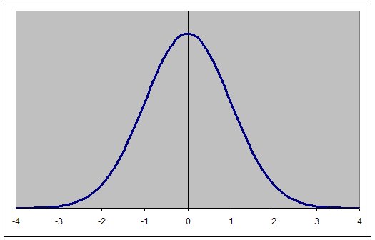
1.Introduction: Examine this graph representing the Normal Curve or a Bell Curve of the level of population of a species, in a certain area, or the density. If you think of the blue line here representing the number of individuals of animals or plants in a population, which exist in an environment with abiotic conditions favoring those at the central value of 0, then you can see that there is actually more positive selection for the central area being exerted than for either of the extremes. Species evolve in much this way. Those having the right amount of insulation, the right amount of ability to survive dessication or drying up, the right abilities to survive in a certain salinity or level of dissolved oxygen, or the right ability to tolerate a high level of wind in their environment, are the ones who are more successful in reproducing and thus their traits get passed along to more offspring. So the X-axis can represent the abiotic variables in an environment.

2. Correlate the month of occurrence of a species and the population levels for that month.

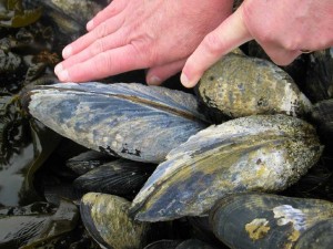
3. We can see from the assignment on abiotic factors, that there may be dozens of such graphs you could make for any organism.musshand At Race Rocks, we have two species of the molluscs called mussels. They are Mytilus californianus and Mytilus trossulus . Visualize the x-axis above being a scale of temperature, for a marine animal such as a mussel, lets say the ideal temperature for mussels is 10 degrees C. Draw a similar graph with 10 in place of the 0 . Show the scale going up and down from 10. Lets say that the Mytilus californianus mussels cannot reproduce at a temperature higher than 12 degrees nor lower than 8 degrees C, so the blue line tapers down and ends at 8 degrees C.
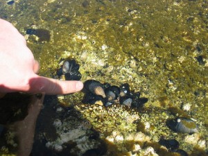
4. Now plot another graph on the same scale, This one is for the other local mussel, Mytilus trossulus. musselpool4It lives in the intermediate level tidepools and can survive in water up to 16 degrees and down to 4 degrees. In the sample above we say that the M.californianus is a Stenothermal ( narrow range of tolerance to heat) animal, whereas the M.trossulus is a Eurythermal (wide range of tolerance to heat) organism
5. Next we will do a similar plot for salinity. Here 30 parts per thousand for salinity becomes the central measurement and above and below that amount make the rest of the scale. M.Californianus prefers to live in water that is 27 parts per thousand. But it can live in up to 30 or down to 25. M.trossulus also prefers 27 parts per thousand, but can live in water that ranges from 32 down to 22 parts per thousand. Now if we combine the same prefixes: Eury and Steno,with the word haline, we will get a word that describes the organisms. So now you have two new words that help describe the variation the same abiotic factor can have on two closely related species.
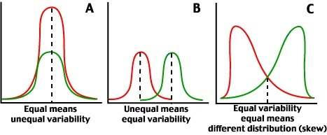
6. Natural Selection which can lead to the evolution of separate species, is often determined by the way an organism is able to tolerate variations in the abiotic factors of it’s environment.variabilityJust when that seemed so straightforward, we have to recognize that selection pressure may affect the same species group in different ways. Two species of mussel may on the other hand prefer different ranges of temperature or salinty instead of the 10 degrees. The picture B could represent that situation. What would the skewed distribution in C therefore represent in terms of selective pressures on the population?

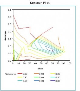
mus7. The Ecological Niche is defined by limiting abiotic and biotic factors: In this assignment, we deal with the problem of defining what are the ideal conditions for an organism’s existence. At Race Rocks, the position on a shoreline within a few centimeters can determine survival of an organism. Use these references to find out about how you can model an ecological niche of an organism. Choose an organism in your own ecosystem and produce a graph representing it’s ecological niche.


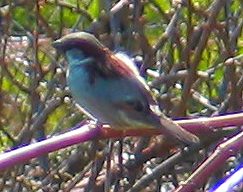
malesparrow8.This now brings us to a classical study in Adaptation which was done over a century ago! This study has provided the data for many studies on limiting factors of the environment. However, be careful about jumping to conclusions! This study points out the difficulties in attributing what may at first seem to be a simple cause and effect relationship. See Bumpus’ Sparrows

9. Extension Materials: Central Tendency and Variability

Also, you may wish to take this opportunity to get into an exercise on Standard Deviation. To draw such a curve as the Normal Curve at the top of the page, one needs to specify two parameters, the mean and the standard deviation.  The graph has a mean of zero and a standard deviation of 1, i.e., (m=0, s=1).  A Normal distribution with a mean of zero and a standard deviation of 1 is also known as the Standard Normal Distribution.

Elassochirus tenuimanus The Race Rocks Taxonomy

Domain Eukarya
Kingdom Animalia
Phylum Arthroppoda
Class Malacostraca
Order Decapoda
Family Paguridae
Genus Elassochirus
Species tenuimanus
Common Name: Wide-hand hermit crab

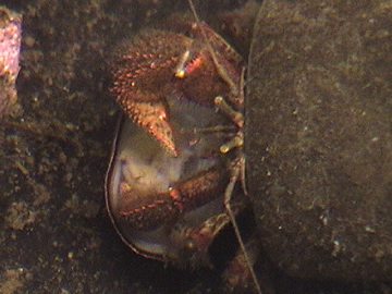
In this video, Elassochirus has been disturbed from eating a limpet (Collisella instabilis). It recovers and returns to eating. Note the colouration of the appendages of the hermit crab. Also note that one arm is much wider than the other. The Collisella which normally has a pale shell, is encrusted with the pink algae Lithothamnion.

General Description:
Named as wide-hand, this species hermit crab has a large and flattened right side of chela, carpus and propodus more than its left side. The right cheliped has a wider carpus than it is long. The walking legs have colours of white, reddish brown and purplish-blue on its merus.

Size:
The exterior length is up to 42 mm (1.6 inches).

Natural History, Habitat and geographical and depth range:
Mud, sand, shell bottoms, and especially rocks. The depth range is intertidal (infrequently) to 388 m (1272 feet). For the geographical range, the hermit crab lives in Bering Sea and Aleutian Islands, from Alaska to Washington, and the northwestern Pacific.
Ovigerous females in Washington usually appear from August to May.  Larvae produce from March to May and Planktonic are in last months of the year.

Behavior
When the animal retreats inside, the right claw is used to block the access to the shell itself. The crab bents this claw beneath the body while walking.

References:
– Pacific Coast Crab and Shrimps, Gregory C. Jensen; Sea Challengers Monterey, California, 1995.

– Marine Invertebrate of the Pacific Northwest, Eugene N. Kozloff; University of Washington Press, Seattle and London, 1996.

http://people.wwc.edu/staff/cowlda/KeyToSpecies/Arthropoda/Crustacea/Malacostraca/Eumalacostraca/
Eucarida/Decapoda/Anomura/Family_Paguridae/Elassochirus_tenuimanus.html


ARCHIVE of Education in the Race Rocks Ecological Reserve

In this file, photos are presented which link to a number of the field labs and other educational applications of Lester B. Pearson College that have taken place at Race Rocks in past years.

Biology Class 1999
Env Systems TIdepool lab 1999
Royal Roads Field Trip
Env Systems 1999
Biology Class 1999
Env Systems 1998 Biology Field Lab 1998 Diving Activity: Schools Project. Group 4 projects 1998
Environmental Systems
Transect Lab on Peg 15 , 1998
Env Systems 1997 Diving Schools activity OUTPOST video Drogue lab : Currents
Environmental Systems Class
Tidepool Study , 1997
Environmental Systems
Current Study 1996
Env Systems 1996
Env Systems 1995
Diving : Schoools project Biology Field Lab 2004
Diving
education- research
Pearson College and Diving at Race Rocks

Lightning as an Abiotic Factor at Race Rocks

Lightning is a very rare occurrence on this part of the Pacific North West Coast, however we show below a method of recording lightning strikes which can be used to compare with other regions of North America. The unusual thing about lightning is that it can occur here in the Strait of Juan de Fuca in what is the winter months in North America. When lightning is never recorded in the interior…at least of Canada.
We are interested in noting Lightning as an abiotic factor because it contributes to the sum total of Atmospheric Nitrogen Fixation and is therefore an important feature for all organisms which are dependent on nutrients from the Nitrogen Cycle. Nitrogen fixation involves Nitrogen, which is a relatively inert gas, which is plentiful in air, being made to combine chemically with other elements to form more reactive nitrogen compounds such as ammonia, nitrates, or nitrites.
This space is reserved for the first person to record a lightning strike from the remote control cameras at Race Rocks!
OBJECTIVES: After doing this assignment, students will be able to:a) Find out where lightning strikes are presently occurring in North America.
b) Evaluate the importance of lightning in the Nitrogen Cycle.
c) Enumerate the other abiotic effects on organisms of lightning strikes.

Procedure:1. The enormous energy of lightning breaks nitrogen molecules and enables their atoms to combine with oxygen in the air forming nitrogen oxides. These dissolve in rain, forming nitrates, that are carried to the earth. Atmospheric nitrogen fixation probably contributes some 5– 8% of the total nitrogen fixed. See the table below for a comparison of sources of Nitrogen Fixation. The major conversion of N2 into ammonia, and thence into proteins, is achieved by microorganisms in the process called nitrogen fixation (or dinitrogen fixation). Give examples of how this process is essential for life. Include the connection between the muscle in your arm and the process of Nitrogen Fixation.

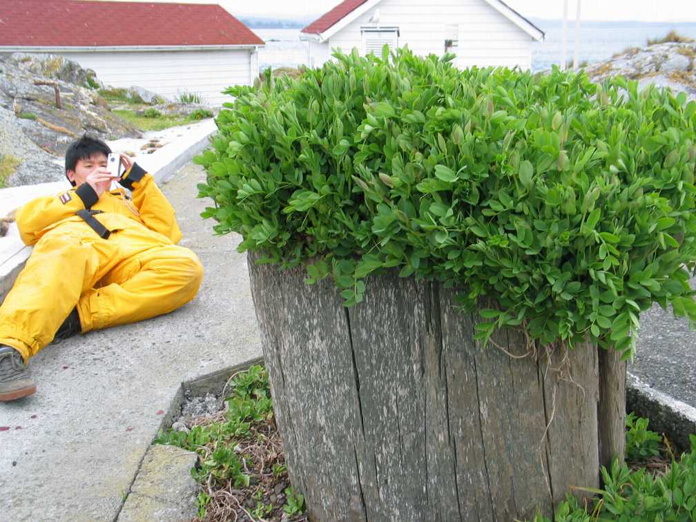
In this picture.. Alex Chan PC yr 32 is trying to get the nitrogen fixing Lathyrus or Beach Pea lined up with Tower at Race Rocks. Check the Beach Pea file to see how well he did.

2.See the file on Biogeochemical Cycles , and construct a Nitrogen cycle from the Race Rocks image clips.

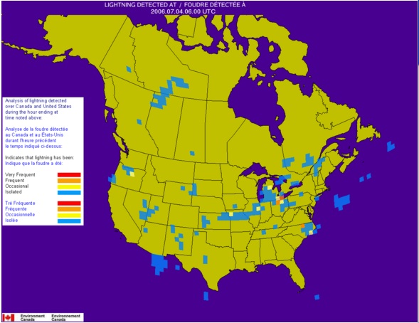
3. The Weather Office of the Government of Canada presents updates of the lightning strikes in North America

Record the Frequency and Location of Lightning strikes on three separate days when you view this link.

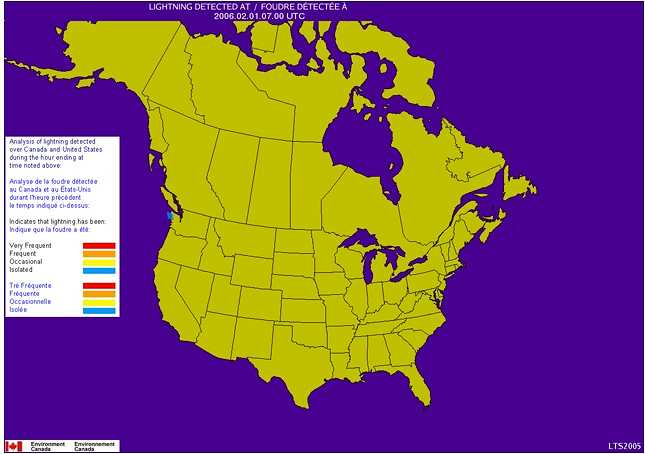
4. Click on the prerecorded sample maps below which show the location and intensity of lightning strikes in the area of the Strait of Juan de Fuca over the period of an hour. In the legend to the left, the estimated frequency of Lightning is depicted as flashes per 1000 square km* per minute as follows:

  • Very Frequent (Red) = more than 6 per minute
  • Frequent (Orange) = 3.0-5.9 per minute
  • Occasional (Yellow) = 1.5-2.9 per minute
  • Isolated (Blue) = less than 1.4 per minute

Note*: 1000 square km represents a circle having a radius of 17.8 km

In the image to the right, you can see the contrast in frequency and intensity of strikes on a July evening. “>
January 31, 2006 2300 hrs
July 3, 2006 1100hrs
The Data below is from various sources, and has been compiled by DF Bezdicek & AC Kennedy, in Microorganisms in Action (eds. JM Lynch & JE Hobbie). Blackwell Scientific Publications 1998. It appears in the website: The Microbial World: N2 fixed (1012 g per year, or 106 metric tons per year)
Type of Fixation
Non-Biological
Industrial about 50
Combustion
about 20
Lightning————–Compare with these other sources ——————-> about 10
Total about 80
Biological
Agricultural land
about 90
Forest and non-agricultural land
about 50
Sea
about 35
Total about 175
5. Extension..for further investigation: Find out why lightning is rare in the winter time in North America, but common in many areas in the summer. If you are from one of these areas that experience many lightning strikes, determine why they are abundant in some areas and not in others. Might you advance an hypothesis on how seasonal differences in Lightning Strikes could affect productivity of plants?( You might want to consider what grows in winter before you jump to conclusions here!)

Abiotic Factors Project

Student Guide
Orientation
Have you noticed reports in the media about climate change and loss of species diversity?Have you ever encountered a special location which has a unique set of organisms that one doesn’t see anywhere else?Have you ever wondered why within a very short distance, the types of animal and plant communities can change entirely, whereas in other areas, one can go for hundred of kilometers without a change of species composition?Have you ever tried to make a plant grow where you want it to grow but find out it keeps dieing?We are slowly becoming aware that in order to preserve a species , we have to be sure the ecosystem of which it is a part is preserved intact..This project will enable students to contribute to a project which may help to shed some light on the questions above. We hope it becomes something that anyone can do long after they get the introduction through this exercise.
OBJECTIVES:1. Present hypotheses on the effect of an abiotic factor on the distribution of an organism, and data which supports the hypothesis.

2. Present evidence for why species change is predicted to be the result of climate change.

3. Relate the occurrence of climate change to species extinction.

4. Analyze the historic records for sea water temperature to see if you can find evidence for climate change.

5.Use the remote control camera to record the effects of weather extremes and correlate these with real time weather data.

PROCEDURE:

1. Introduction: On the website racerocks.ca, we have made an effort to show the relationships between species distribution and abiotic factors. Separate files for nine atmospheric factors and 8 ocean related factors are available from this environmental data index page: Take some time to familiarize yourself with the wide range of abiotic factors which we are recording at Race Rocks and at the files which show how those abiotic effects effect the organisms of the environment. Your task in this assignment is to record a graph of a weather event and correlate it with an image of the environmental response captured from the remote control cameras.  See this file on Correlation Investigations

2. Wind Speed and Direction, are very significant factors in this kind of Coastal Ecosystem. Studies on correlations of barometric pressure and wind speed are also suggested in the Correlation File 

3, Barometric Pressure and the Effect on Organisms: There is some question as to whether organisms can sense changing barometric pressure. Click on this file about barometric pressure and evaluate the evidence that scientists use to show that some organisms do have the ability to detect changing barometric pressures. What is the adaptive advantage of this ability? You may, with careful observation of animal behavior, come up with some evidence either supporting or rejecting this ability. On the racerocks.com weather station, track the weather at Race Rocks for a week. Within that time note the behaviour of animals when the barometer graph is peaking and then dropping . Can you establish a correlation between activity and impending storms?
Hint: to quantify, select a number of times from the graph when the wind is at it’s peak, and the barometer is at a low. Is there always a time lag, if so how much?.

4. Lightning as an Abiotic Factor:
Some of the factors are much more important than others. For example: Lightning is of minor importance most of the time at Race Rocks, or for that matter, anywhere in the local Strait of Juan de Fuca area, compared to wind speed and direction.
Use the link on the lightning page to find out where lightning is presently occurring in North America. Calculate the frequency of lightning strikes and the area which is affected for any one viewing session. Find out from the reference about the abiotic effects of Lightning, about one of the important effects of Lightning related to Nutrient Cycles . There are obviously other abiotic effects of lightning. List two that you can come up with here.
If you can take a screen shot in the summer of this map showing lightning in the Strait of Juan de Fuca, enter it as an observation on the OceanQuest GIS sighting record.5. 5. Change Through Time:
The records of Salinity and Temperature have been collected by the lightkeepers at Race Rocks up to 1977 and by the Marine Protected Area Guardians from that time to the present. These records provide a valuable insight into how factors can remain stable or change over time. See the Archive of Seawater Temperature and Salinity 1921-present


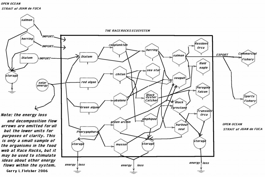
THE ENERGY FLOW ASSIGNMENT

OBJECTIVES: After doing this assignment, you will be able to:a) Trace the pathway of the flow of energy in a portion of the Race Rocks Ecological Reserve.

b) Use a symbolic model to represent energy flow in your own ecosystem.

c) Discuss the contributions of the Odum brothers to the science of Ecology.

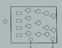
PROCEDURE:1.Energy Flow in the Ecosystems of Race Rocks can be partially represented by the figure1.Click on any of the boxes to see the organism which is part of the energy flow and the food web of the Islands.
2. You will have seen that some of the links, especially for the top level consumers have videos and slide shows of energy flow in action involving the predators at Race Rocks. Some of these images have been submitted by viewers using the remote camera 5 .
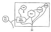
Your challenge is to come up with a picture or a set of pictures which show energy flow in action. Watch the seabirds on the island, especially in the summer during nesting season as they deliver food to chicks. At low tide, you can often see shorebirds like the Black oyster-catcher as it hammers away at intertidal invertebrates for food. Use the OceanQuest GIS sighting report process to add your observation to the records.3. Use this blank template to construct an energy flow model for your observation.( For further information on the definition of the symbols, see #4 below. You can eliminate most of the boxes, just include ones for which you have direct evidence.4.This is a link to a resource which outlines the theory of modelling energy flow with odum symbols. You may also use it for further ideas that will help you in the construction of an energy flow diagram your own ecosystem.

5. Extension material: Investigate the work of the Odum brothers, in material linked at the bottom of the reference in #4. Write a paragraph on the significance of their work for the modern understanding of Ecology.

6..Extension Material: Investigate the application of the Odum Energy Flow Models in the reference below on the Ebro Watershed.


Figure 1: Energy Flow at Race Rocks…click on the symbols below

For Further Reference on the application of this model: External Link: Models of Energy Flow for Rural Planning in the Ebro River Watershed